Stable count distribution
In probability theory, the stable count distribution is the conjugate prior of a one-sided stable distribution. This distribution was discovered by Stephen Lihn (Chinese: 藺鴻圖) in his 2017 study of daily distributions of the S&P 500 and the VIX.[1] The stable distribution family is also sometimes referred to as the Lévy alpha-stable distribution, after Paul Lévy, the first mathematician to have studied it.[2]
|
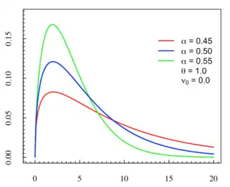
Probability density function  | |||
|
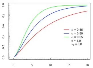
Cumulative distribution function  | |||
| Parameters |
∈ (0, 1) — stability parameter | ||
|---|---|---|---|
| Support | x ∈ R and x ∈ [, ∞) | ||
| CDF | integral form exists | ||
| Mean | |||
| Median | not analytically expressible | ||
| Mode | not analytically expressible | ||
| Variance | |||
| Skewness | TBD | ||
| Ex. kurtosis | TBD | ||
| MGF | Fox-Wright representation exists | ||
Of the three parameters defining the distribution, the stability parameter is most important. Stable count distributions have . The known analytical case of is related to the VIX distribution (See Section 7 of [1]). All the moments are finite for the distribution.
Definition
Its standard distribution is defined as
where and
Its location-scale family is defined as
where , , and
In the above expression, is a one-sided stable distribution,[3] which is defined as following.
Let be a standard stable random variable whose distribution is characterized by , then we have
where .
Consider the Lévy sum where , then has the density where . Set , we arrive at without the normalization constant.
The reason why this distribution is called "stable count" can be understood by the relation . Note that is the "count" of the Lévy sum. Given a fixed , this distribution gives the probability of taking steps to travel one unit of distance.
Integral form
Based on the integral form of and , we have the integral form of as
Based on the double-sine integral above, it leads to the integral form of the standard CDF:
where Failed to parse (SVG (MathML can be enabled via browser plugin): Invalid response ("Math extension cannot connect to Restbase.") from server "http://localhost:6011/en.wikipedia.org/v1/":): {\displaystyle \text{Si}(x)=\int_0^x \frac{\sin(x)}{x}\,dx} is the sine integral function.
The Wright representation
In "Series representation", it is shown that the stable count distribution is a special case of the Wright function (See Section 4 of [4]):
This leads to the Hankel integral: (based on (1.4.3) of [5])
- where Ha represents a Hankel contour.
Alternative derivation – lambda decomposition
Another approach to derive the stable count distribution is to use the Laplace transform of the one-sided stable distribution, (Section 2.4 of [1])
- where .
Let , and one can decompose the integral on the left hand side as a product distribution of a standard Laplace distribution and a standard stable count distribution,
where .
This is called the "lambda decomposition" (See Section 4 of [1]) since the LHS was named as "symmetric lambda distribution" in Lihn's former works. However, it has several more popular names such as "exponential power distribution", or the "generalized error/normal distribution", often referred to when . It is also the Weibull survival function in Reliability engineering.
Lambda decomposition is the foundation of Lihn's framework of asset returns under the stable law. The LHS is the distribution of asset returns. On the RHS, the Laplace distribution represents the lepkurtotic noise, and the stable count distribution represents the volatility.
Stable Vol distribution
A variant of the stable count distribution is called the stable vol distribution . The Laplace transform of can be re-expressed in terms of a Gaussian mixture of (See Section 6 of [4]). It is derived from the lambda decomposition above by a change of variable such that
where
This transformation is named generalized Gauss transmutation since it generalizes the Gauss-Laplace transmutation, which is equivalent to .
Connection to Gamma and Poisson distributions
The shape parameter of the Gamma and Poisson Distributions is connected to the inverse of Lévy's stability parameter . The upper regularized gamma function can be expressed as an incomplete integral of as
By replacing with the decomposition and carrying out one integral, we have:
Reverting back to , we arrive at the decomposition of in terms of a stable count:
Differentiate by , we arrive at the desired formula:
This is in the form of a product distribution. The term in the RHS is associated with a Weibull distribution of shape . Hence, this formula connects the stable count distribution to the probability density function of a Gamma distribution (here) and the probability mass function of a Poisson distribution (here, ). And the shape parameter can be regarded as inverse of Lévy's stability parameter .
Connection to Chi and Chi-squared distributions
The degrees of freedom in the chi and chi-squared Distributions can be shown to be related to . Hence, the original idea of viewing as an integer index in the lambda decomposition is justified here.
For the chi-squared distribution, it is straightforward since the chi-squared distribution is a special case of the gamma distribution, in that . And from above, the shape parameter of a gamma distribution is .
For the chi distribution, we begin with its CDF , where . Differentiate by , we have its density function as
This formula connects with through the term.
Connection to generalized Gamma distributions
The generalized gamma distribution is a probability distribution with two shape parameters, and is the super set of the gamma distribution, the Weibull distribution, the exponential distribution, and the half-normal distribution. Its CDF is in the form of . (Note: We use instead of for consistency and to avoid confusion with .) Differentiate by , we arrive at the product-distribution formula:
where denotes the PDF of a generalized gamma distribution, whose CDF is parametrized as . This formula connects with through the term. The term is an exponent representing the second degree of freedom in the shape-parameter space.
This formula is singular for the case of a Weibull distribution since must be one for ; but for to exist, must be greater than one. When , is a delta function and this formula becomes trivial. The Weibull distribution has its distinct way of decomposition as following.
Connection to Weibull distribution
For a Weibull distribution whose CDF is , its shape parameter is equivalent to Lévy's stability parameter .
A similar expression of product distribution can be derived, such that the kernel is either a one-sided Laplace distribution or a Rayleigh distribution . It begins with the complementary CDF, which comes from Lambda decomposition:
By taking derivative on , we obtain the product distribution form of a Weibull distribution PDF as
where and . it is clear that from the and terms.
Asymptotic properties
For stable distribution family, it is essential to understand its asymptotic behaviors. From,[3] for small ,
This confirms .
For large ,
This shows that the tail of decays exponentially at infinity. The larger is, the stronger the decay.
This tail is in the form of a generalized gamma distribution, where in its parametrization, , , and . Hence, it is equivalent to , whose CDF is parametrized as .
Moments
The n-th moment of is the -th moment of . All positive moments are finite. This in a way solves the thorny issue of diverging moments in the stable distribution. (See Section 2.4 of [1])
The analytic solution of moments is obtained through the Wright function:
where (See (1.4.28) of [5])
Thus, the mean of is
The variance is
And the lowest moment is by applying when .
The n-th moment of the stable vol distribution is
Moment generating function
The MGF can be expressed by a Fox-Wright function or Fox H-function:
As a verification, at , (see below) can be Taylor-expanded to via .
Known analytical case – quartic stable count
When , is the Lévy distribution which is an inverse gamma distribution. Thus is a shifted gamma distribution of shape 3/2 and scale ,
where , .
Its mean is and its standard deviation is . This called "quartic stable count distribution". The word "quartic" comes from Lihn's former work on the lambda distribution[6] where . At this setting, many facets of stable count distribution have elegant analytical solutions.
The p-th central moments are . The CDF is where is the lower incomplete gamma function. And the MGF is . (See Section 3 of [1])
Special case when α → 1
As becomes larger, the peak of the distribution becomes sharper. A special case of is when . The distribution behaves like a Dirac delta function,
where , and .
Likewise, the stable vol distribution at also becomes a delta function,
Series representation
Based on the series representation of the one-sided stable distribution, we have:
- .
This series representation has two interpretations:
- First, a similar form of this series was first given in Pollard (1948),[7] and in "Relation to Mittag-Leffler function", it is stated that where is the Laplace transform of the Mittag-Leffler function .
- Secondly, this series is a special case of the Wright function : (See Section 1.4 of [5])
The proof is obtained by the reflection formula of the Gamma function: , which admits the mapping: in . The Wright representation leads to analytical solutions for many statistical properties of the stable count distribution and establish another connection to fractional calculus.
Applications
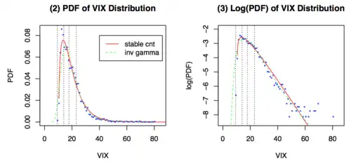
Stable count distribution can represent the daily distribution of VIX quite well. It is hypothesized that VIX is distributed like with and (See Section 7 of [1]). Thus the stable count distribution is the first-order marginal distribution of a volatility process. In this context, is called the "floor volatility". In practice, VIX rarely drops below 10. This phenomenon justifies the concept of "floor volatility". A sample of the fit is shown below:

One form of mean-reverting SDE for is based on a modified Cox–Ingersoll–Ross (CIR) model. Assume is the volatility process, we have
where is the so-called "vol of vol". The "vol of vol" for VIX is called VVIX, which has a typical value of about 85.[8]
This SDE is analytically tractable and satisfies the Feller condition, thus would never go below . But there is a subtle issue between theory and practice. There has been about 0.6% probability that VIX did go below . This is called "spillover". To address it, one can replace the square root term with , where provides a small leakage channel for to drift slightly below .
Extremely low VIX reading indicates a very complacent market. Thus the spillover condition, , carries a certain significance - When it occurs, it usually indicates the calm before the storm in the business cycle.
Generation of Random Variables
As the modified CIR model above shows, it takes another input parameter to simulate sequences of stable count random variables. The mean-reverting stochastic process takes the form of
which should produce that distributes like as . And is a user-specified preference for how fast should change.
By solving the Fokker-Planck equation, the solution for in terms of is
It can also be written as a ratio of two Wright functions,
When , this process is reduced to the modified CIR model where . This is the only special case where is a straight line.
Likewise, if the asymptotic distribution is as , the solution, denoted as below, is
When , it is reduced to a quadratic polynomial: .
Stable Extension of the CIR Model
By relaxing the rigid relation between the term and the term above, the stable extension of the CIR model can be constructed as
which is reduced to the original CIR model at : . Hence, the parameter controls the mean-reverting speed, the location parameter sets where the mean is, is the volatility parameter, and is the shape parameter for the stable law.
By solving the Fokker-Planck equation, the solution for the PDF at is
To make sense of this solution, consider asymptotically for large , 's tail is still in the form of a generalized gamma distribution, where in its parametrization, , , and . It is reduced to the original CIR model at where with and ; hence .
Fractional calculus
Relation to Mittag-Leffler function
From Section 4 of,[9] the inverse Laplace transform of the Mittag-Leffler function is ()
On the other hand, the following relation was given by Pollard (1948),[7]
Thus by , we obtain the relation between stable count distribution and Mittag-Leffter function:
This relation can be verified quickly at where and . This leads to the well-known quartic stable count result:
Relation to time-fractional Fokker-Planck equation
The ordinary Fokker-Planck equation (FPE) is , where is the Fokker-Planck space operator, is the diffusion coefficient, is the temperature, and is the external field. The time-fractional FPE introduces the additional fractional derivative such that , where is the fractional diffusion coefficient.
Let in , we obtain the kernel for the time-fractional FPE (Eq (16) of [10])
from which the fractional density can be calculated from an ordinary solution via
Since via change of variable , the above integral becomes the product distribution with , similar to the "lambda decomposition" concept, and scaling of time :
Here is interpreted as the distribution of impurity, expressed in the unit of , that causes the anomalous diffusion.
See also
References
- Lihn, Stephen (2017). "A Theory of Asset Return and Volatility Under Stable Law and Stable Lambda Distribution". SSRN 3046732.
- Paul Lévy, Calcul des probabilités 1925
- Penson, K. A.; Górska, K. (2010-11-17). "Exact and Explicit Probability Densities for One-Sided Lévy Stable Distributions". Physical Review Letters. 105 (21): 210604. arXiv:1007.0193. Bibcode:2010PhRvL.105u0604P. doi:10.1103/PhysRevLett.105.210604. PMID 21231282. S2CID 27497684.
- Lihn, Stephen (2020). "Stable Count Distribution for the Volatility Indices and Space-Time Generalized Stable Characteristic Function". SSRN 3659383.
- Mathai, A.M.; Haubold, H.J. (2017). Fractional and Multivariable Calculus. Springer Optimization and Its Applications. Vol. 122. Cham: Springer International Publishing. doi:10.1007/978-3-319-59993-9. ISBN 9783319599922.
- Lihn, Stephen H. T. (2017-01-26). "From Volatility Smile to Risk Neutral Probability and Closed Form Solution of Local Volatility Function". Rochester, NY. doi:10.2139/ssrn.2906522. S2CID 157746678. SSRN 2906522.
{{cite journal}}: Cite journal requires|journal=(help) - Pollard, Harry (1948-12-01). "The completely monotonic character of the Mittag-Leffler function $E_a \left( { - x} \right)$". Bulletin of the American Mathematical Society. 54 (12): 1115–1117. doi:10.1090/S0002-9904-1948-09132-7. ISSN 0002-9904.
- "DOUBLE THE FUN WITH CBOE's VVIX Index" (PDF). www.cboe.com. Retrieved 2019-08-09.
- Saxena, R. K.; Mathai, A. M.; Haubold, H. J. (2009-09-01). "Mittag-Leffler Functions and Their Applications". arXiv:0909.0230 [math.CA].
- Barkai, E. (2001-03-29). "Fractional Fokker-Planck equation, solution, and application". Physical Review E. 63 (4): 046118. Bibcode:2001PhRvE..63d6118B. doi:10.1103/PhysRevE.63.046118. ISSN 1063-651X. PMID 11308923. S2CID 18112355.
External links
- R Package 'stabledist' by Diethelm Wuertz, Martin Maechler and Rmetrics core team members. Computes stable density, probability, quantiles, and random numbers. Updated Sept. 12, 2016.