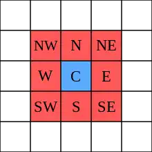
Moore neighborhood
In cellular automata, the Moore neighborhood is defined on a two-dimensional square lattice and is composed of a central cell and the eight cells that surround it.

Name
The neighborhood is named after Edward F. Moore, a pioneer of cellular automata theory.
Importance
It is one of the two most commonly used neighborhood types, the other one being the von Neumann neighborhood, which excludes the corner cells. The well known Conway's Game of Life, for example, uses the Moore neighborhood. It is similar to the notion of 8-connected pixels in computer graphics.
The Moore neighbourhood of a cell is the cell itself and the cells at a Chebyshev distance of 1.
The concept can be extended to higher dimensions, for example forming a 26-cell cubic neighborhood for a cellular automaton in three dimensions, as used by 3D Life. In dimension d, where , the size of the neighborhood is 3d − 1.
In two dimensions, the number of cells in an extended Moore neighbourhood of range r is (2r + 1)2.
Algorithm
The idea behind the formulation of Moore neighborhood is to find the contour of a given graph. This idea was a great challenge for most analysts of the 18th century, and as a result an algorithm was derived from the Moore graph which was later called the Moore Neighborhood algorithm.
The pseudocode for the Moore-Neighbor tracing algorithm is
Input: A square tessellation, T, containing a connected component P of black cells.
Output: A sequence B (b1, b2, ..., bk) of boundary pixels i.e. the contour.
Define M(a) to be the Moore neighborhood of pixel a.
Let p denote the current boundary pixel.
Let c denote the current pixel under consideration i.e. c is in M(p).
Let b denote the backtrack of c (i.e. neighbor pixel of p that was previously tested)

Begin
  Set B to be empty.
  From bottom to top and left to right scan the cells of T until a black pixel, s, of P is found.
  Insert s in B.
  Set the current boundary point p to s i.e. p=s
  Let b = the pixel from which s was entered during the image scan.
  Set c to be the next clockwise pixel (from b) in M(p).
  While c not equal to s do
    If c is black
      insert c in B
      Let b = p
      Let p = c
      (backtrack: move the current pixel c to the pixel from which p was entered)
      Let c = next clockwise pixel (from b) in M(p).
    else
      (advance the current pixel c to the next clockwise pixel in M(p) and update backtrack)
      Let b = c
      Let c = next clockwise pixel (from b) in M(p).
    end If
  end While
End
Termination condition
The original termination condition was to stop after visiting the start pixel for the second time. This limits the set of contours the algorithm will walk completely. An improved stopping condition proposed by Jacob Eliosoff is to stop after entering the start pixel for the second time in the same direction you originally entered it.
References
- Weisstein, Eric W. "Moore Neighborhood". MathWorld.
- Tyler, Tim, The Moore neighborhood at cell-auto.com