Growth accounting
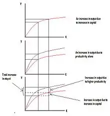
Growth accounting is a procedure used in economics to measure the contribution of different factors to economic growth and to indirectly compute the rate of technological progress, measured as a residual, in an economy.[1] Growth accounting decomposes the growth rate of an economy's total output into that which is due to increases in the contributing amount of the factors used—usually the increase in the amount of capital and labor—and that which cannot be accounted for by observable changes in factor utilization. The unexplained part of growth in GDP is then taken to represent increases in productivity (getting more output with the same amounts of inputs) or a measure of broadly defined technological progress.
The technique has been applied to virtually every economy in the world and a common finding is that observed levels of economic growth cannot be explained simply by changes in the stock of capital in the economy or population and labor force growth rates. Hence, technological progress plays a key role in the economic growth of nations, or the lack of it.
History
This methodology was introduced by Robert Solow and Trevor Swan in 1957.[2][3] Growth accounting was proposed for management accounting in the 1980s.[4][5] but they did not gain on as management tools. The reason is clear. The production functions are understood and formulated differently in growth accounting and management accounting. In growth accounting the production function is formulated as a function OUTPUT=F (INPUT), which formulation leads to maximize the average productivity ratio OUTPUT/INPUT. Average productivity has never been accepted in management accounting (in business) as a performance criterion or an objective to be maximized because it would mean the end of the profitable business. Instead the production function is formulated as a function INCOME=F(OUTPUT-INPUT) which is to be maximized. The name of the game is to maximize income, not to maximize productivity or production.[6]: 6
Abstract example

The growth accounting model is normally expressed in the form of the exponential growth function. As an abstract example consider an economy whose total output (GDP) grows at 3% per year. Over the same period its capital stock grows at 6% per year and its labor force by 1%. The contribution of the growth rate of capital to output is equal to that growth rate weighted by the share of capital in total output and the contribution of labor is given by the growth rate of labor weighted by labor's share in income. If capital's share in output is 1⁄3, then labor's share is 2⁄3 (assuming these are the only two factors of production). This means that the portion of growth in output which is due to changes in factors is .06×(1⁄3)+.01×(2⁄3)=.027 or 2.7%. This means that there is still 0.3% of the growth in output that cannot be accounted for. This remainder is the increase in the productivity of factors that happened over the period, or the measure of technological progress during this time.
Specific example
Growth accounting can also be expressed in the form of the arithmetical model, which is used here because it is more descriptive and understandable. The principle of the accounting model is simple. The weighted growth rates of inputs (factors of production) are subtracted from the weighted growth rates of outputs. Because the accounting result is obtained by subtracting it is often called a "residual". The residual is often defined as the growth rate of output not explained by the share-weighted growth rates of the inputs.[7]: 6
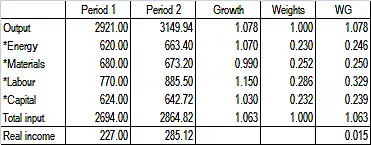
We can use the real process data of the production model in order to show the logic of the growth accounting model and identify possible differences in relation to the productivity model. When the production data is the same in the model comparison the differences in the accounting results are only due to accounting models. We get the following growth accounting from the production data.

The growth accounting procedure proceeds as follows. First is calculated the growth rates for the output and the inputs by dividing the Period 2 numbers with the Period 1 numbers. Then the weights of inputs are computed as input shares of the total input (Period 1). Weighted growth rates (WG) are obtained by weighting growth rates with the weights. The accounting result is obtained by subtracting the weighted growth rates of the inputs from the growth rate of the output. In this case the accounting result is 0.015 which implies a productivity growth by 1.5%.
We note that the productivity model reports a 1.4% productivity growth from the same production data. The difference (1.4% versus 1.5%) is caused by the different production volume used in the models. In the productivity model the input volume is used as a production volume measure giving the growth rate 1.063. In this case productivity is defined as follows: output volume per one unit of input volume. In the growth accounting model the output volume is used as a production volume measure giving the growth rate 1.078. In this case productivity is defined as follows: input consumption per one unit of output volume. The case can be verified easily with the aid of productivity model using output as a production volume.
The accounting result of the growth accounting model is expressed as an index number, in this example 1.015, which depicts the average productivity change. As demonstrated above we cannot draw correct conclusions based on average productivity numbers. This is due to the fact that productivity is accounted as an independent variable separated from the entity it belongs to, i.e. real income formation. Hence, if we compare in a practical situation two growth accounting results of the same production process we do not know which one is better in terms of production performance. We have to know separately income effects of productivity change and production volume change or their combined income effect in order to understand which one result is better and how much better.
This kind of scientific mistake of wrong analysis level has been recognized and described long ago.[8] Vygotsky cautions against the risk of separating the issue under review from the total environment, the entity of which the issue is an essential part. By studying only this isolated issue we are likely to end up with incorrect conclusions. A second practical example illustrates this warning. Let us assume we are studying the properties of water in putting out a fire. If we focus the review on small components of the whole, in this case the elements oxygen and hydrogen, we come to the conclusion that hydrogen is an explosive gas and oxygen is a catalyst in combustion. Therefore, their compound water could be explosive and unsuitable for putting out a fire. This incorrect conclusion arises from the fact that the components have been separated from the entity.[9]: 10
Technical derivation
The total output of an economy is modeled as being produced by various factors of production, with capital and labor being the primary ones in modern economies (although land and natural resources can also be included). This is usually captured by an aggregate production function:[10]
where Y is total output, K is the stock of capital in the economy, L is the labor force (or population) and A is a "catch all" factor for technology, role of institutions and other relevant forces which measures how productively capital and labor are used in production.
Standard assumptions on the form of the function F(.) is that it is increasing in K, L, A (if you increase productivity or you increase the number of factors used you get more output) and that it is homogeneous of degree one, or in other words that there are constant returns to scale (which means that if you double both K and L you get double the output). The assumption of constant returns to scale facilitates the assumption of perfect competition which in turn implies that factors get their marginal products:
where MPK denotes the extra units of output produced with an additional unit of capital and similarly, for MPL. Wages paid to labor are denoted by w and the rate of profit or the real interest rate is denoted by r. Note that the assumption of perfect competition enables us to take prices as given. For simplicity we assume unit price (i.e. P =1), and thus quantities also represent values in all equations.
If we totally differentiate the above production function we get;
where denotes the partial derivative with respect to factor i, or for the case of capital and labor, the marginal products. With perfect competition this equation becomes:
If we divide through by Y and convert each change into growth rates we get:
or denoting a growth rate (percentage change over time) of a factor as we get:
Then is the share of total income that goes to capital, which can be denoted as and is the share of total income that goes to labor, denoted by . This allows us to express the above equation as:
In principle the terms , , and are all observable and can be measured using standard national income accounting methods (with capital stock being measured using investment rates via the perpetual inventory method). The term however is not directly observable as it captures technological growth and improvement in productivity that are unrelated to changes in use of factors. This term is usually referred to as Solow residual or Total factor productivity growth. Slightly rearranging the previous equation we can measure this as that portion of increase in total output which is not due to the (weighted) growth of factor inputs:
Another way to express the same idea is in per capita (or per worker) terms in which we subtract off the growth rate of labor force from both sides:
which states that the rate of technological growth is that part of the growth rate of per capita income which is not due to the (weighted) growth rate of capital per person.
Notes and references
- Sickles, R., & Zelenyuk, V. (2019). Measurement of Productivity and Efficiency: Theory and Practice. Cambridge: Cambridge University Press. doi:10.1017/9781139565981
- Solow, Robert (1957). "Technical change and the aggregate production function". Review of Economics and Statistics. 39 (3): 312–320. doi:10.2307/1926047. JSTOR 1926047.
- Spencer, Barbara (2008). "Trevor Swan And The Neoclassical Growth Model". History of Political Economy. 42.
- Loggerenberg van, B.; Cucchiaro, S. (1982). "Productivity Measurement and the Bottom Line". National Productivity Review. 1 (1): 87–99. doi:10.1002/npr.4040010111.
- Bechler, J.G (1984). "The Productivity Management Process". American Productivity Center.
{{cite journal}}: Cite journal requires|journal=(help) - Kohli, U (2012). Productivity: National vs. Domestic (PDF). Sydney, Australia: EMG Workshop, University of New South Wales, November 21–23, 2012.
- Hulten, C.R. (September 2009). "Growth Accounting" (PDF). NATIONAL BUREAU OF ECONOMIC RESEARCH. doi:10.3386/w15341.
{{cite journal}}: Cite journal requires|journal=(help) - Vygotsky, L. (1962). Thought and Language. MIT Press (original work 1934).
- Saari, S. (2011). Production and Productivity as Sources of Well-being. MIDO OY. p. 25.
- Zelenyuk (2014). "Testing Significance of Contributions in Growth Accounting, with Application to Testing ICT Impact on Labor Productivity of Developed Countries". International Journal of Business and Economics. 13 (2): 115–126.