Expected linear time MST algorithm

Each iteration of the algorithm relies on an adaptation of Borůvka's algorithm referred to as a Borůvka step:

 Input: A graph G with no isolated vertices
   1 For each vertex v, select the lightest edge incident on v 
   2 Create a contracted graph G' by replacing each component of G connected by the edges selected in step 1 with a single vertex
   3 Remove all isolated vertices, self-loops, and non-minimal repetitive edges from G' 
 Output: The edges selected in step 1 and the contracted graph G'

A Borůvka step is equivalent to the inner loop of Borůvka's algorithm, which runs in O(m) time where m is the number of edges in G. Furthermore, since each edge can be selected at most twice (once by each incident vertex) the maximum number of disconnected components after step 1 is equal to half the number of vertices. Thus, a Borůvka step reduces the number of vertices in the graph by at least a factor of two and deletes at least n/2 edges where n is the number of vertices in G.

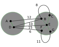
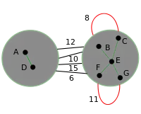
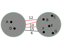
Example execution of a Borůvka step

Image	Description
	The lightest edge incident on each vertex is highlighted in green.
	The graph is contracted and each component connected by the edges selected in step 1 is replaced by a single vertex. This creates two supernodes. All edges from the original graph remain.
	Edges that form self loops to the supernodes are deleted.
	Non-minimal redundant edges between supernodes are deleted.
	The result of one Borůvka Step on the sample graph is a graph with two supernodes connected by a single edge.

In each iteration the algorithm removes edges with particular properties that exclude them from the minimum spanning tree. These are called F-heavy edges and are defined as follows. Let F be a forest on the graph H. An F-heavy edge is an edge e connecting vertices u,v whose weight is strictly greater than the weight of the heaviest edge on the path from u to v in F. (If a path does not exist in F it is considered to have infinite weight). Any edge that is not F-heavy is F-light. If F is a subgraph of G then any F-heavy edge in G cannot be in the minimum spanning tree of G by the cycle property. Given a forest, F-heavy edges can be computed in linear time using a minimum spanning tree verification algorithm.[2][3]

Lemma- Let H be a subgraph of G formed by including each edge of G independently with probability p and let F be the minimum spanning forest of H. The expected number of F-light edges in G is at most n/p where n is the number of vertices in G.

To prove the lemma examine the edges of G as they are being added to H. The number of F-light edges in G is independent of the order in which the edges of H are selected since the minimum spanning forest of H is the same for all selection orders. For the sake of the proof consider selecting edges for H by taking the edges of G one at a time in order of edge weight from lightest to heaviest. Let e be the current edge being considered. If the endpoints of e are in two disconnected components of H then e is the lightest edge connecting those components and if it is added to H it will be in F by the cut property. This also means e is F-light regardless of whether or not it is added to H since only heavier edges are subsequently considered. If both endpoints of e are in the same component of H then it is (and always will be) F-heavy by the cycle property. Edge e is then added to H with probability p.

The maximum number of F-light edges added to H is n-1 since any minimum spanning tree of H has n-1 edges. Once n-1 F-light edges have been added to H none of the subsequent edges considered are F-light by the cycle property. Thus, the number of F-light edges in G is bounded by the number of F-light edges considered for H before n-1 F-light edges are actually added to H. Since any F-light edge is added with probability p this is equivalent to flipping a coin with probability p of coming up heads until n-1 heads have appeared. The total number of coin flips is equal to the number of F-light edges in G. The distribution of the number of coin flips is given by the inverse binomial distribution with parameters n-1 and p. For these parameters the expected value of this distribution is (n-1)/p.

Ignoring work done in recursive subproblems the total amount of work done in a single invocation of the algorithm is linear in the number of edges in the input graph. Step 1 takes constant time. Borůvka steps can be executed in time linear in the number of edges as mentioned in the Borůvka step section. Step 3 iterates through the edges and flips a single coin for each one so it is linear in the number of edges. Step 4 can be executed in linear time using a modified linear time minimum spanning tree verification algorithm.[2][3] Since the work done in one iteration of the algorithm is linear in the number of edges the work done in one complete run of the algorithm (including all recursive calls) is bounded by a constant factor times the total number of edges in the original problem and all recursive subproblems.

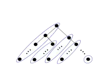
Each invocation of the algorithm produces at most two subproblems so the set of subproblems forms a binary tree. Each Borůvka step reduces the number of vertices by at least a factor of two so after two Borůvka steps the number of vertices has been reduced by a factor of four. Thus, if the original graph has n vertices and m edges then at depth d of the tree each subproblem is on a graph of at most n/4^d vertices. Also the tree has at most log₄n levels.

Left paths of a binary tree are circled in blue

To reason about the recursion tree let the left child problem be the subproblem in the recursive call in step 3 and the right child problem be the subproblem in the recursive call in step 5. Count the total number of edges in the original problem and all subproblems by counting the number of edges in each left path of the tree. A left path begins at either a right child or the root and includes all nodes reachable through a path of left children. The left paths of a binary tree are shown circled in blue in the diagram on the right.

Each edge in a left child problem is selected from the edges of its parent problem (less the edges contracted in the Borůvka steps) with probability 1/2. If a parent problem has x edges then the expected number of edges in the left child problem is at most x/2. If x is replaced by a random variable X then by the linearity of expectation the expected number of edges in the left child problem Y is given by ${\displaystyle E[Y]\leq E[X]/2}$. Thus if the expected number of edges in a problem at the top of a left path is k then the sum of the expected number of edges in each subproblem in the left path is at most ${\displaystyle \sum _{d=0}^{\infty }{\frac {k}{2^{d}}}=2k}$ (see Geometric series). The root has m edges so the expected number of edges is equal to 2m plus twice the expected number of edges in each right subproblem.

The expected number of edges in each right subproblem is equal to the number of F-light edges in the parent problem where F is the minimum spanning tree of the left subproblem. The number of F-light edges is less than or equal to twice the number of vertices in the subproblem by the sampling lemma. The number of vertices in a subproblem at depth d is n/4^d so the total number of vertices in all right subproblems is given by ${\displaystyle \sum _{d=1}^{\infty }{\frac {2^{d-1}n}{4^{d}}}=n/2}$. Thus, the expected number of edges in the original problem and all subproblems is at most 2m+n. Since n at most 2m for a graph with no isolated vertices the algorithm runs in expected time O(m).

The worst case runtime is equivalent to the runtime of Borůvka's algorithm. This occurs if all edges are added to either the left or right subproblem on each invocation. In this case the algorithm is identical to Borůvka's algorithm which runs in O(min{n², mlogn}) on a graph with n vertices and m edges.

References

- Karger, David R.; Klein, Philip N.; Tarjan, Robert E. (1995). "A randomized linear-time algorithm to find minimum spanning trees". Journal of the ACM. 42 (2): 321. CiteSeerX 10.1.1.39.9012. doi:10.1145/201019.201022. S2CID 832583.
- Dixon, Brandon; Rauch, Monika; Tarjan, Robert E. (1992). "Verification and Sensitivity Analysis of Minimum Spanning Trees in Linear Time". SIAM Journal on Computing. 21 (6): 1184. CiteSeerX 10.1.1.49.25. doi:10.1137/0221070.
- King, Valerie (1995). A Simpler Minimum Spanning Tree Verification Algorithm. Proceedings of the 4th International Workshop on Algorithms and Data Structures. London, UK, UK: Springer-Verlag. pp. 440–448.