Derivation using cumulated distribution function ${\displaystyle F_{X}}$

At first, we limit ourselves to f whose derivative is never 0 (thus, f is a diffeomorphism). Then, the inverse map ${\displaystyle f^{-1}}$ exists and f is either monotonically increasing or monotonically decreasing.

If f is monotonically increasing, then ${\displaystyle x\leq f^{-1}(y)\Leftrightarrow f(x)\leq f(f^{-1}(y))=y}$ and ${\displaystyle f^{\prime }>0}$. Therefore:

${\displaystyle {\begin{array}{rcl}\varrho _{Y}(y)&=&{\frac {d}{dy}}P(f(X)\leq y)={\frac {d}{dy}}P(X\leq f^{-1}(y))\\&=&{\frac {d}{dy}}F_{X}(f^{-1}(y))=\varrho _{X}(f^{-1}(y)){\frac {df^{-1}(y)}{dy}}\end{array}}}$

If f is monotonically decreasing, then ${\displaystyle x\leq f^{-1}(y)\Leftrightarrow f(x)\geq f(f^{-1}(y))=y}$ and ${\displaystyle f^{\prime }<0}$. Therefore:

${\displaystyle {\begin{array}{rcl}\varrho _{Y}(y)&=&{\frac {d}{dy}}P(f(X)\leq y)={\frac {d}{dy}}P(X\geq f^{-1}(y))\\&=&{\frac {d}{dy}}\left(1-F_{X}(f^{-1}(y))\right)=-\varrho _{X}(f^{-1}(y)){\frac {df^{-1}(y)}{dy}}\end{array}}}$

This can be summarized as:

${\displaystyle \varrho _{Y}(y)={\begin{cases}0,&{\text{if }}y\notin f(\mathbb {R} )\\\varrho _{X}(f^{-1}(y))\cdot \left|{\frac {df^{-1}(y)}{dy}}\right|,&{\text{if }}y\in f(\mathbb {R} )\end{cases}}}$

(5)

If now the derivative ${\displaystyle f^{\prime }(x_{i})=0}$ does vanish at some positions ${\displaystyle x_{i}}$, ${\displaystyle i=1,\ldots ,N}$, then we split the definition space of f using those position into ${\displaystyle N+1}$ disjoint intervals ${\displaystyle I_{j}}$. Equation 5 holds for the functions ${\displaystyle f_{I_{j}}}$ limited in their definition space to those intervals ${\displaystyle I_{j}}$. We have

${\displaystyle {\begin{array}{rcl}P(f(X)\leq y)&=&\sum \limits _{j=1}^{N+1}P(f_{I_{j}}(X)\leq y)\\\varrho _{Y}(y)={\frac {d}{dy}}P(f(X)\leq y)&=&\sum \limits _{j=1}^{N+1}\varrho _{X}(f_{I_{j}}^{-1}(y))\cdot \left|{\frac {df_{I_{j}}^{-1}(y)}{dy}}\right|\end{array}}}$

With the convention that the sum over 0 addends is 0 and using the inverse function theorem, it is possible to write this in a more compact form (read as: sum over all x, where f(x)=y):

ℝ → ℝ mapping ${\displaystyle \varrho _{Y}(y)=\sum \limits _{x,f(x)=y}{\frac {\varrho _{X}(x)}{\left|f^{\prime }(x)\right|}}}$

(6)

Derivation using Integral Substitution

In this section we consider a different derivation.

The probability in 4 is the integral over the probability density. Again in the case of monotonically increasing f, we have:

${\displaystyle {\begin{array}{rcl}\int _{-\infty }^{y}\varrho _{Y}(u)\,du&=&P(Y\leq y)=P(f(X)\leq y)=P(X\leq f^{-1}(y))\\&=&\int _{-\infty }^{f^{-1}(y)}\varrho _{X}(x)\,dx\end{array}}}$

Now we substitute u = f(x) in the integral on the right hand site, i.e. ${\displaystyle x=f^{-1}(u)}$ and ${\displaystyle {\frac {du}{dx}}=f^{\prime }(x)}$. The integral limits are then from -∞ to y and in the rule “${\displaystyle dx={\frac {dx}{du}}\,du}$” we have ${\displaystyle {\frac {dx}{du}}={\frac {d\,f^{-1}(u)}{du}}}$ due to the inverse function theorem. Consequentially:

${\displaystyle \int _{-\infty }^{y}\varrho _{Y}(u)\,du=\int _{-\infty }^{y}\varrho _{X}(f^{-1}(u))\,{\frac {d\,f^{-1}(u)}{du}}\,du}$

Taking the derivative of both sides with respect to y, we get:

${\displaystyle \varrho _{Y}(y)=\varrho _{X}(f^{-1}(y))\,{\frac {d\,f^{-1}(y)}{dy}}}$

Following the same argument as in the last section, we can again derive equation 6.

This rule often misleads physics books to present the following viewpoint, which might be easier to remember, but is not mathematically sound: If you multiply the probability density ${\displaystyle \varrho _{X}(x)}$ with the “infinitesimal length” ${\displaystyle dx}$, then you will get the probability ${\displaystyle \varrho _{X}(x)\,dx}$ for X to lie in the interval [x, x+dx]. Changing to new coordinates y, you will get by substitution:

${\displaystyle \varrho _{X}(x)\,dx=\underbrace {\varrho _{X}(x(y))\,{\frac {dx}{dy}}} _{\varrho _{Y}(y)}\,dy}$

Derivation using the Delta Distribution

In this section we consider another different derivation, often used in physics.

We start again with equation 4 and write this as an integral:

${\displaystyle {\begin{array}{rcl}\varrho _{Y}(y)&=&{\frac {d}{dy}}P(f(X)\leq y)\\&=&{\frac {d}{dy}}\int _{\{x\in \mathbb {R} \mid f(x)\leq y\}}\,\varrho _{X}(x)\,dx\\&=&{\frac {d}{dy}}\int _{\mathbb {R} }\Theta (y-f(x))\,\varrho _{X}(x)\,dx\\&=&\int _{\mathbb {R} }{\frac {d}{dy}}\Theta (y-f(x))\,\varrho _{X}(x)\,dx\\&=&\int _{\mathbb {R} }\delta (y-f(x))\,\varrho _{X}(x)\,dx\end{array}}}$

The intuitive interpretation of the last expression is: one integrates over all possible x-values and uses the delta “function” to pick all positions where y = f(x). This formula is often found in physics books, possibly written as expectation value, ${\displaystyle \langle \ldots \rangle }$:

ℝ → ℝ mapping (using Dirac Delta Distribution) ${\displaystyle \varrho _{Y}(y)=\int _{\mathbb {R} }\delta (y-f(x))\,\varrho _{X}(x)\,dx=\langle \,\delta (y-f(x))\,\rangle \;.}$

(7)

We can see this formula is equivalent to equation 6 using the following identity

${\displaystyle \int _{\mathbb {R} }\delta (h(x))\,g(x)\,dx=\sum \limits _{x,h(x)=0}{\frac {g(x)}{\left|h^{\prime }(x)\right|}}}$

Examples

• Let us consider the following specific example: let ${\displaystyle \varrho _{X}(x)={\frac {\exp[-0.5x^{2}]}{\sqrt {2\pi }}}}$ and ${\displaystyle f(x)=x^{2}}$. We choose to use equation 6 (equations 5 and 7 lead to the same result). We calculate the derivative ${\displaystyle f^{\prime }(x)=2x}$ and find all x for which f(x)=y, which are ${\displaystyle -{\sqrt {y}}}$ and ${\displaystyle +{\sqrt {y}}}$ if y>0 and none otherwise. For y>0 we have:

${\displaystyle \varrho _{Y}(y)=\sum \limits _{x,f(x)=y}{\frac {\varrho _{X}(x)}{\left|f^{\prime }(x)\right|}}={\frac {\varrho _{X}(-{\sqrt {y}})}{\left|f^{\prime }(-{\sqrt {y}})\right|}}+{\frac {\varrho _{X}(+{\sqrt {y}})}{\left|f^{\prime }(+{\sqrt {y}})\right|}}={\frac {\exp[-0.5y]}{{\sqrt {2\pi }}\,2{\sqrt {y}}}}+{\frac {\exp[-0.5y]}{{\sqrt {2\pi }}\,2{\sqrt {y}}}}={\frac {\exp[-0.5y]}{\sqrt {2\pi \,y}}}}$

Since f never reaches negative values, the sum remains 0 for y<0 and we finally obtain:

${\displaystyle \varrho _{Y}(y)={\begin{cases}0,&{\text{if }}y\leq 0\\{\frac {\exp[-0.5y]}{\sqrt {2\pi \,y}}},&{\text{if }}y>0\end{cases}}}$

This example is illustrated in the following graphics:

Random numbers are generated according to the standard normal distribution X ~ N(0,1). They are shown on the x-axis of figure (a). Many of them are around 0. Each of those numbers is mapped according to y = x², which is shown with grey arrows for two example points. For many generated realisations of X, a histogram on the y-axis will converge towards the wanted probability density function ρ_Y shown in (c). In order to analytically derive this function, we start by observing that in order for Y to be between any v and v+Δv, X must have been between either ${\displaystyle -{\sqrt {v+\Delta v}}}$ and ${\displaystyle -{\sqrt {v}}}$, or, between ${\displaystyle {\sqrt {v}}}$ and ${\displaystyle {\sqrt {v+\Delta v}}}$. Those intervals are marked in figures (b) and (c). Because the probability is equal to the area under the probability density function, we can determine ρ_Y from the condition that the grey shaded area in (c) must be equal to the sum of the areas in (b). The areas are calculated using integrals and it is useful to take the limit ${\displaystyle \Delta v\to 0}$ in order to get the formula noted in (c).

• Another example is the inverse transformation method. Suppose a computer generates random numbers X with a uniform distribution on [0, 1], i.e.

${\displaystyle \varrho _{X}(x)\equiv {\begin{cases}1,&{\text{if }}0\leq x\leq 1\\0,&{\text{else.}}\end{cases}}}$

If we want to obtain random numbers according to a distribution with the pdf ${\displaystyle \varrho _{Z}}$, we choose f as the inverse function of the cdf of Z, i.e. ${\displaystyle Y=f(X)=F_{Z}^{-1}(X)}$. We can now show that Y will have the same distribution as the wanted Z, ${\displaystyle \varrho _{Y}=\varrho _{Z}}$ by using equation 5 and the fact that ${\displaystyle f^{-1}=F_{Z}}$:

${\displaystyle {\begin{array}{rcl}\varrho _{Y}(y)&=&{\begin{cases}0,&{\text{if }}y\notin F_{Z}^{-1}(\mathbb {R} )\\\varrho _{X}(F_{Z}(y))\cdot \left|{\frac {dF_{Z}(y)}{dy}}\right|,&{\text{if }}y\in F_{Z}^{-1}(\mathbb {R} )\end{cases}}\\&=&1\cdot \left|{\frac {dF_{Z}(y)}{dy}}\right|=\varrho _{Z}(y)\end{array}}}$.

An example is illustrated in the following plot:

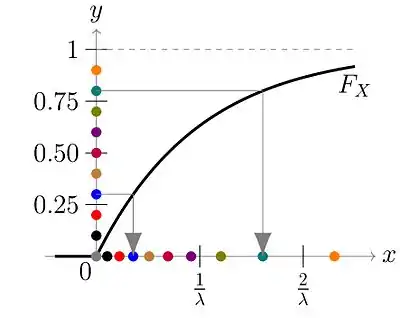Random numbers y_i are generated from a uniform distribution between 0 and 1, i.e. Y ~ U(0, 1). They are sketched as colored points on the y-axis. Each of the points is mapped according to x=F^-1(y), which is shown with gray arrows for two example points. In this example, we have used an exponential distribution. Hence, for x ≥ 0, the probability density is ${\displaystyle \varrho _{X}(x)=\lambda e^{-\lambda \,x}}$ and the cumulated distribution function is ${\displaystyle F(x)=1-e^{-\lambda \,x}}$. Therefore, ${\displaystyle x=F^{-1}(y)=-{\frac {\ln(1-y)}{\lambda }}}$. We can see that using this method, many points end up close to 0 and only few points end up having high x-values - just as it is expected for an exponential distribution.

Examples

• Let ${\displaystyle Y=f({\vec {X}})=X_{1}+X_{2}}$ with the independent, continuous random variable X₁ and X₂. According to equation 9, we have:

${\displaystyle {\begin{array}{rcl}\varrho _{Y}(y)&=&{\frac {d}{dy}}\int _{\mathbb {R} }\varrho _{X_{2}}(x_{2})\int _{\mathbb {R} }\varrho _{X_{1}}(x_{1})\,\delta (y-x_{2}-x_{1})\,dx_{1}\,dx_{2}\\&=&\int _{\mathbb {R} }\varrho _{X_{2}}(x_{2})\,\varrho _{X_{1}}(y-x_{2})\,dx_{2}\end{array}}}$

If one uses the sum formula instead, the sum runs over all x₁, for which ${\displaystyle f({\vec {x}})=x_{1}+x_{2}=y}$, i.e. where x₁ = y - x₂.

The derivative is ${\displaystyle {\frac {\partial (x_{1}+x_{2})}{\partial x_{1}}}=1}$, so that one also obtains the equation ${\displaystyle \varrho _{Y}(y)=\int _{\mathbb {R} }\varrho _{X_{2}}(x_{2})\,\varrho _{X_{1}}(y-x_{2})\,dx_{2}}$.

Integrating over x₂ first leads to the following, equivalent expression:

${\displaystyle \varrho _{Y}(y)=\int _{\mathbb {R} }\varrho _{X_{1}}(x_{1})\,\varrho _{X_{2}}(y-x_{1})\,dx_{1}}$

• If ${\displaystyle Y=X_{1}-X_{2}}$ with independent X₁ and X₂, then ${\displaystyle \varrho _{Y}(y)=\int _{\mathbb {R} }\varrho _{X_{1}}(x_{1})\,\varrho _{X_{2}}(x_{1}-y)\,dx_{1}}$.

• If ${\displaystyle Y=X_{1}\cdot X_{2}}$ with independent X₁ and X₂, then ${\displaystyle \varrho _{Y}(y)=\int _{\mathbb {R} }\varrho _{X_{1}}(x_{1})\,\varrho _{X_{2}}\left({\frac {y}{x_{1}}}\right){\frac {1}{|x_{1}|}}\,dx_{1}}$.

• If ${\displaystyle Y={\frac {X_{1}}{X_{2}}}}$ with independent X₁ and X₂, then ${\displaystyle \varrho _{Y}(y)=\int _{\mathbb {R} }\varrho _{X_{1}}(x_{2}\cdot y)\,\varrho _{X_{2}}(x_{2})\,|x_{2}|\,dx_{2}}$.

• Given the independent random variables X₁ and X₂ with the density

${\displaystyle \varrho _{\vec {X}}(x_{1},x_{2})={\begin{cases}1/\pi ,&{\text{if }}x_{1}^{2}+x_{2}^{2}\leq 1\\0,&{\text{otherwise}}\end{cases}}}$

Let ${\displaystyle Y:={\sqrt {X_{1}^{2}+X_{2}^{2}}}}$. According to equation 8, we need to solve:

${\displaystyle \varrho _{Y}(y)={\frac {d}{dy}}\int _{{\bigl \{}{\vec {x}}\in \mathbb {R} ^{n}\mid {\sqrt {x_{1}^{2}+x_{2}^{2}}}\,\leq \,y{\bigr \}}}\,{\frac {1}{\pi }}\,dx_{1}\,dx_{2}}$

The last integral is over a circle with radius y ≤ 1, hence with the area ${\displaystyle \pi y^{2}}$. This simplifies the calculation:

${\displaystyle 0\leq y\leq 1\Rightarrow \varrho _{Y}(y)={\frac {1}{\pi }}\,{\frac {d}{dy}}(\pi y^{2})={\frac {2\pi \,y}{\pi }}=2y}$.

If y<0, we integrate over an empty set, which gives 0. If y>1, ${\displaystyle \varrho _{\vec {X}}=0}$. Therefore, the final result is:

${\displaystyle \varrho _{Y}(y)={\begin{cases}2y,&{\text{if }}0\leq y\leq 1\\0,&{\text{otherwise}}\end{cases}}}$

This example is illustrated in the following graphics:

Figure (a) shows a sketch of random sample points from a uniform distribution in a circle of radius 1, subdivided into rings. In figure (b), we count how many of those points fell into each of the rings with the same width Δv. Since the area of the rings increases linearly with the radius, one can expect more points for larger radii. For Δv → 0, the normalized histogram in (b) will converge to the wanted probability density function ρ_Y. In order to calculate ρ_Y analytically, we first derive the cumulated distribution function F_Y, plotted in figure (d). F_Y(y) is the probability to find a point inside the circle of radius v (shown in grey in figure (c)). For v between 0 and 1, we find ${\displaystyle F_{Y}(v)={\frac {A_{v}}{A_{tot}}}={\frac {\pi v^{2}}{\pi 1^{2}}}=v^{2}}$. The slope of F_Y is the wanted probability density function ${\displaystyle \rho _{Y}(y)={\frac {dF_{Y}(y)}{dy}}=2y}$, in agreement with figure (b).

Examples

• Given the random vector ${\displaystyle {\vec {X}}}$ and the invertible matrix A and a vector ${\displaystyle {\vec {b}}}$, let ${\displaystyle {\vec {Y}}=A{\vec {X}}^{T}+{\vec {b}}}$. Then ${\displaystyle \varrho _{\vec {Y}}({\vec {y}})=\varrho _{\vec {X}}\left(A^{-1}\,({\vec {y}}-{\vec {b}})\right)\;\left|\det A^{-1}\right|}$. Also, ${\displaystyle \det A^{-1}=1/\det A}$.
• Given the independent random variables ${\displaystyle X_{1}}$ and ${\displaystyle X_{2}}$, we introduce polar coordinates ${\displaystyle Y_{1}={\sqrt {X_{1}^{2}+X_{2}^{2}}}}$ and ${\displaystyle Y_{2}=\operatorname {atan2} (X_{2},X_{1})}$. The inverse map is ${\displaystyle X_{1}=Y_{1}\,\cos Y_{2}}$ and ${\displaystyle X_{2}=Y_{1}\,\sin Y_{2}}$. Due to Jacobian determinant ${\displaystyle y_{1}}$, the wanted density is ${\displaystyle \varrho _{\vec {Y}}(y_{1},y_{2})=y_{1}\,\varrho _{\vec {X}}(y_{1}\,\cos y_{2},\;y_{1}\,\sin y_{2})}$.

Independent Target-Components

If one knows beforehand that the components of ${\displaystyle Y_{i}}$ will be independent, i.e.

${\displaystyle \varrho _{\vec {Y}}(y_{1},\ldots ,y_{n})=\varrho _{Y_{1}}(y_{1})\cdot \ldots \cdot \varrho _{Y_{n}}(y_{n})\;,}$

then the density ${\displaystyle \varrho _{Y_{i}}}$ of each component ${\displaystyle Y_{i}=f_{i}({\vec {X}})}$ can be calculated like in the above section Mapping of a Random Vector to a Random Variable.

Split Integral Region

Sometimes it is useful to split the integral region in equation 3 into parts that can be evaluate separately. This can be made explicit by rewriting 3 with delta functions:

${\displaystyle \varrho _{\vec {Y}}({\vec {y}})=\int _{\mathbb {R} ^{n}}\varrho _{\vec {X}}({\vec {x}})\,\delta (y_{1}-f({\vec {x}})_{1})\cdot \ldots \cdot \delta (y_{m}-f({\vec {x}})_{m})\,d^{n}x}$

and then use the identity ${\displaystyle \delta (x-x_{0})=\int _{\mathbb {R} }\delta (x-\xi )\,\delta (\xi -x_{0})\,d\xi }$.

Helper Coordinates

If f is injective, then it can be easier to introduce additional helper coordinates Y_m+1 to Y_n, then do the ${\displaystyle \mathbb {R} ^{n}\to \mathbb {R} ^{n}}$ transformation from section Invertible Transformation of a Random Vector and finally integrate out all helper coordinates of the so-obtained density.

Statistical Physics

• Suppose atoms in a laser are moving with normally distributed velocities V_x, ${\displaystyle \varrho _{V_{x}}(v_{x})={\frac {\exp[-v_{x}^{2}/2\sigma ^{2}]}{\sqrt {2\pi \sigma ^{2}}}}}$, σ² = k_BT/m. Due to the Doppler effect, light emitted with frequency f₀ by an atom moving with v_x will be detected as f ≈ f₀ ( 1 + v_x / c ). Hence, f is a function of V_x. What does the detected spectrum, ${\displaystyle \varrho _{f}}$, look like? (Answer: Gaussian around f₀.)
• Suppose the velocity components of an ideal gas (V_x, V_y, V_z) are identically, independently normally distributed as in the last example. What is the probability density ${\displaystyle \varrho _{V}}$ of ${\displaystyle V={\sqrt {V_{x}^{2}+V_{y}^{2}+V_{z}^{2}}}}$? (The answer is known as Maxwell-Boltzmann distribution.)

Quantifying Uncertainty of Derived Properties

• Suppose we do not know the exact value of X and Y, but we can assign a probability distribution to each of them. What is the distrubution of the derived property Z = X² / Y and what is the mean value and standard deviation of Z? (To tackle such problems, linearisation around the mean values are sometimes used and both X and Y are assumed to be normally distributed. However, we are not limited to such restrictions.)
• Suppose we consider the value of one gram gold, silver and platinum in one year from now as independent random variables G, S and P, respectively. Box A contains 1 gram gold, 2 gram silver and 3 gram platinum. Box B contains 4, 5 and 6 gram, respectively. Thus, ${\displaystyle {\begin{pmatrix}A\\B\end{pmatrix}}={\begin{pmatrix}1&2&3\\4&5&6\end{pmatrix}}{\begin{pmatrix}G\\S\\P\end{pmatrix}}}$. What is the value of the contents in box A (or box B) in one year from now? (The answer is given in an example above.) Note that A and B are correlated.

Note that the above examples assume the distribution of ${\displaystyle {\vec {X}}}$ to be known. If it is unknown, or if the calculation is based on only a few data points, methods from mathematical statistics are a better choice to quantify uncertainty.

Generation of Correlated Random Numbers

Correlated random numbers can be obtained by first generating a vector of uncorrelated random numbers and then applying a function on them.

• In order to obtain random numbers with covariance matrix C_Y, we can use the following know procedure: Calculate the Cholesky decomposition C_Y = A A^T. Generate a vector ${\displaystyle {\vec {x}}}$ of uncorrelated random numbers with all var(X_i) = 1. Apply the matrix A: ${\displaystyle {\vec {Y}}=A{\vec {X}}}$. This will result in correlated random variables with covariance matrix C_Y = A A^T.

• With the formulas outlined in this Wikibook, we can additionally study the shape of the resulting distribution and the effect of non-linear transformations. Consider, e.g., that X is uniform distributed in [0, 2π], Y₁ = sin(X) and Y₂ = cos(X). In this case, a 2D plot of random numbers from (Y₁, Y₂) will show a uniform distribution on a circle. Although Y₁ and Y₂ are stochastically dependent, they are uncorrelated. It is therefore important to know the resulting distribution, because ${\displaystyle \varrho _{\vec {Y}}(y_{1},y_{1})}$ has more information than the covariance matrix C_Y.