QuTiP
QuTiP, short for the Quantum Toolbox in Python, is an open-source computational physics software library for simulating quantum systems, particularly open quantum systems.[1][2] QuTiP allows simulation of Hamiltonians with arbitrary time-dependence, allowing simulation of situations of interest in quantum optics, ion trapping, superconducting circuits and quantum nanomechanical resonators. The library includes extensive visualization facilities for content under simulations.
 | |
| Stable release | 4.7.0
/ February 8, 2022 |
|---|---|
| Preview release | 5.0.0.dev
|
| Written in | Python |
| Platform | Cross-platform |
| Type | Library |
| License | BSD 3-clause |
| Website | qutip |
QuTiP's API provides a Python interface and uses Cython to allow run-time compilation and extensions via C and C++. QuTiP is built to work well with popular Python packages NumPy, SciPy, Matplotlib and IPython.
History
The idea for the QuTip project was conceived in 2010 by PhD student Paul Nation, who was using the quantum optics toolbox for MATLAB in his research. According to Paul Nation, he wanted to create a python package similar to qotoolbox because he "was not a big fan of MATLAB" and then decided to "just write it [him]self".[3] As a postdoctoral fellow, at the RIKEN Institute in Japan, he met Robert Johansson and the two worked together on the package. In contrast to its predecessor qotoolbox, which relies on the proprietary MATLAB environment, it was published in 2012 under an open source license.[2]
The Version created by Nation and Johansson already contained the most important features of the package, but QuTips scope and features are constantly being extended by a large community of contributors.[4] It has grown in popularity amongst physicists, with over 250.000 downloads in the year 2021.[5]
Examples
Creating quantum objects
>>> import qutip
>>> import numpy as np
>>> psi=qutip.Qobj([[0.6],[0.8]]) # create quantum state from a list
>>> psi
Quantum object: dims = [[2], [1]], shape = (2, 1), type = ket
Qobj data =
[[0.6]
 [0.8]]
>>> phi=qutip.Qobj(np.array([0.8,-0.6])) # create quantum state from a numpy-array
>>> phi
Quantum object: dims = [[2], [1]], shape = (2, 1), type = ket
Qobj data =
[[ 0.8]
 [-0.6]]
>>> e0=qutip.basis(2,0) # create a basis vector
>>> e0
Quantum object: dims = [[2], [1]], shape = (2, 1), type = ket
Qobj data =
[[1.]
 [0.]]
>>> A=qutip.Qobj(np.array([[1,2j],[-2j,1]])) # create quantum operator from numpy array
>>> A
Quantum object: dims = [[2], [2]], shape = (2, 2), type = oper, isherm = True
Qobj data =
[[1.+0.j 0.+2.j]
 [0.-2.j 1.+0.j]]
>>> qutip.sigmay() # some common quantum objects, like pauli matrices, are predefined in the qutip package
Quantum object: dims = [[2], [2]], shape = (2, 2), type = oper, isherm = True
Qobj data =
[[0.+0.j 0.-1.j]
 [0.+1.j 0.+0.j]]
Basic operations
>>> A*qutip.sigmax()+qutip.sigmay() # we can add and multiply quantum objects of compatible shape and dimension
Quantum object: dims = [[2], [2]], shape = (2, 2), type = oper, isherm = False
Qobj data =
[[0.+2.j 1.-1.j]
 [1.+1.j 0.-2.j]]
>>> psi.dag() # hermitian conjugate
Quantum object: dims = [[1], [2]], shape = (1, 2), type = bra
Qobj data =
[[0.6 0.8]]
>>> psi.proj() # projector onto a quantum state
Quantum object: dims = [[2], [2]], shape = (2, 2), type = oper, isherm = True
Qobj data =
[[0.36 0.48]
 [0.48 0.64]]
>>> A.tr() # trace of operator
2.0
>>> A.eigenstates() # diagonalize an operator
(array([-1.,  3.]), array([Quantum object: dims = [[2], [1]], shape = (2, 1), type = ket
       Qobj data =
       [[-0.70710678+0.j        ]
        [ 0.        -0.70710678j]]                                  ,
       Quantum object: dims = [[2], [1]], shape = (2, 1), type = ket
       Qobj data =
       [[-0.70710678+0.j        ]
        [ 0.        +0.70710678j]]                                  ],
      dtype=object))
>>> (1j*A).expm() # matrix exponential of an operator
Quantum object: dims = [[2], [2]], shape = (2, 2), type = oper, isherm = False
Qobj data =
[[-0.2248451-0.35017549j -0.4912955-0.7651474j ]
 [ 0.4912955+0.7651474j  -0.2248451-0.35017549j]]
>>> qutip.tensor(qutip.sigmaz(),qutip.sigmay()) # tensor product
Quantum object: dims = [[2, 2], [2, 2]], shape = (4, 4), type = oper, isherm = True
Qobj data =
[[0.+0.j 0.-1.j 0.+0.j 0.+0.j]
 [0.+1.j 0.+0.j 0.+0.j 0.+0.j]
 [0.+0.j 0.+0.j 0.+0.j 0.+1.j]
 [0.+0.j 0.+0.j 0.-1.j 0.+0.j]]
Time evolution
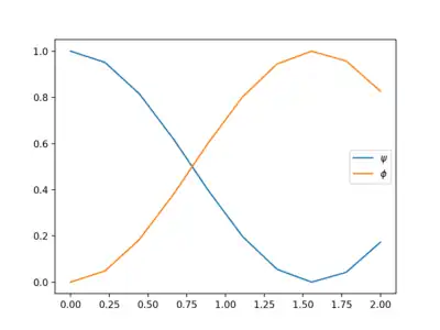
>>> Hamiltonian=qutip.sigmay()
>>> times=np.linspace(0,2,10)
>>> result=qutip.sesolve(Hamiltonian,psi,times,[psi.proj(),phi.proj()]) # unitary time evolution of a system according to schroedinger equation
>>> expectpsi,expectphi=result.expect # expectation values of projectors onto psi and phi
>>> plt.figure(dpi=200)
>>> plt.plot(times,expectpsi)
>>> plt.plot(times,expectphi)
>>> plt.legend([r"$\psi$",r"$\phi$"])
>>> plt.show()
 results of exemplary simulation: probabilities to measure the states and as functions of time.
Simulating a non-unitary time evolution according to the Lindblad Master Equation is possible with the qutip.mesolve function [6]
References
- Johansson, J.R.; Nation, P.D.; Nori, Franco (April 2013). "QuTiP 2: A Python framework for the dynamics of open quantum systems". Computer Physics Communications. 184 (4): 1234–1240. arXiv:1211.6518. Bibcode:2013CoPhC.184.1234J. doi:10.1016/j.cpc.2012.11.019. S2CID 15261366.
- Johansson, J.R.; Nation, P.D.; Nori, Franco (August 2012). "QuTiP: An open-source Python framework for the dynamics of open quantum systems". Computer Physics Communications. 183 (8): 1760–1772. arXiv:1110.0573. Bibcode:2012CoPhC.183.1760J. doi:10.1016/j.cpc.2012.02.021. S2CID 15055747.
- Tobias Macey (24 September 2017). "QuTiP with Paul Nation - Episode 128" (Podcast). Podcast.__init__. Event occurs at 6:15. Retrieved 10 August 2022.
- QuTip Contributors. "QuTiP - Quantum Toolbox in Python". GitHub. Retrieved 11 August 2022.
{{cite web}}:|author=has generic name (help) - The QuTip Admin Team. "QuTiP 2021 Annual Report". GitHub. Retrieved 11 August 2022.
- QuTiP developers and contributors. "Lindblad Master Equation Solver". Retrieved 2022-07-24.