Z-order curve
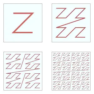
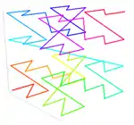
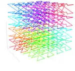
In mathematical analysis and computer science, functions which are Z-order, Lebesgue curve, Morton space-filling curve,[1] Morton order or Morton code map multidimensional data to one dimension while preserving locality of the data points. It is named in France after Henri Lebesgue, who studied it in 1904,[2] and named in the United States after Guy Macdonald Morton, who first applied the order to file sequencing in 1966.[3] The z-value of a point in multidimensions is simply calculated by interleaving the binary representations of its coordinate values. Once the data are sorted into this ordering, any one-dimensional data structure can be used, such as simple one dimensional arrays, binary search trees, B-trees, skip lists or (with low significant bits truncated) hash tables. The resulting ordering can equivalently be described as the order one would get from a depth-first traversal of a quadtree or octree.
Coordinate values
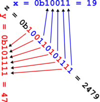
The figure below shows the Z-values for the two dimensional case with integer coordinates 0 ≤ x ≤ 7, 0 ≤ y ≤ 7 (shown both in decimal and binary). Interleaving the binary coordinate values (starting to the right with the x-bit (in blue) and alternating to the left with the y-bit (in red)) yields the binary z-values (tilted by 45° as shown). Connecting the z-values in their numerical order produces the recursively Z-shaped curve. Two-dimensional Z-values are also known as quadkey values.
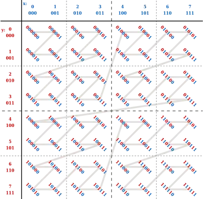
The Z-values of the x coordinates are described as binary numbers from the Moser–de Bruijn sequence, having nonzero bits only in their even positions:
x[] = {0b000000, 0b000001, 0b000100, 0b000101, 0b010000, 0b010001, 0b010100, 0b010101}
The sum and difference of two x values are calculated by using bitwise operations:
x[i+j] = ((x[i] | 0b10101010) + x[j]) & 0b01010101
x[i−j] = ((x[i] & 0b01010101) − x[j]) & 0b01010101  if i ≥ j
This property can be used to offset a Z-value, for example in two dimensions the coordinates to the top (decreasing y), bottom (increasing y), left (decreasing x) and right (increasing x) from the current Z-value z are:
top    = (((z & 0b10101010) − 1) & 0b10101010) | (z & 0b01010101)
bottom = (((z | 0b01010101) + 1) & 0b10101010) | (z & 0b01010101)
left   = (((z & 0b01010101) − 1) & 0b01010101) | (z & 0b10101010)
right  = (((z | 0b10101010) + 1) & 0b01010101) | (z & 0b10101010)
And in general to add two two-dimensional Z-values w and z:
sum = ((z | 0b10101010) + (w & 0b01010101) & 0b01010101) | ((z | 0b01010101) + (w & 0b10101010) & 0b10101010)
Efficiently building quadtrees and octrees
The Z-ordering can be used to efficiently build a quadtree (2D) or octree (3D) for a set of points.[4][5] The basic idea is to sort the input set according to Z-order. Once sorted, the points can either be stored in a binary search tree and used directly, which is called a linear quadtree,[6] or they can be used to build a pointer based quadtree.
The input points are usually scaled in each dimension to be positive integers, either as a fixed point representation over the unit range [0, 1] or corresponding to the machine word size. Both representations are equivalent and allow for the highest order non-zero bit to be found in constant time. Each square in the quadtree has a side length which is a power of two, and corner coordinates which are multiples of the side length. Given any two points, the derived square for the two points is the smallest square covering both points. The interleaving of bits from the x and y components of each point is called the shuffle of x and y, and can be extended to higher dimensions.[4]
Points can be sorted according to their shuffle without explicitly interleaving the bits. To do this, for each dimension, the most significant bit of the exclusive or of the coordinates of the two points for that dimension is examined. The dimension for which the most significant bit is largest is then used to compare the two points to determine their shuffle order.
The exclusive or operation masks off the higher order bits for which the two coordinates are identical. Since the shuffle interleaves bits from higher order to lower order, identifying the coordinate with the largest most significant bit, identifies the first bit in the shuffle order which differs, and that coordinate can be used to compare the two points.[7] This is shown in the following Python code:
def cmp_zorder(lhs, rhs) -> bool:
    """Compare z-ordering."""
    # Assume lhs and rhs array-like objects of indices.
    assert len(lhs) == len(rhs)
    # Will contain the most significant dimension.
    msd = 0
    # Loop over the other dimensions.
    for dim in range(1, len(lhs)):
        # Check if the current dimension is more significant
        # by comparing the most significant bits.
        if less_msb(lhs[msd] ^ rhs[msd], lhs[dim] ^ rhs[dim]):
            msd = dim
    return lhs[msd] < rhs[msd]
One way to determine whether the most significant bit is smaller is to compare the floor of the base-2 logarithm of each point. It turns out the following operation is equivalent, and only requires exclusive or operations:[7]
def less_msb(x: int, y: int) -> bool:
    return x < y and x < (x ^ y)
It is also possible to compare floating point numbers using the same technique. The less_msb function is modified to first compare the exponents. Only when they are equal is the standard less_msb function used on the mantissas.[8]
Once the points are in sorted order, two properties make it easy to build a quadtree: The first is that the points contained in a square of the quadtree form a contiguous interval in the sorted order. The second is that if more than one child of a square contains an input point, the square is the derived square for two adjacent points in the sorted order.
For each adjacent pair of points, the derived square is computed and its side length determined. For each derived square, the interval containing it is bounded by the first larger square to the right and to the left in sorted order.[4] Each such interval corresponds to a square in the quadtree. The result of this is a compressed quadtree, where only nodes containing input points or two or more children are present. A non-compressed quadtree can be built by restoring the missing nodes, if desired.
Rather than building a pointer based quadtree, the points can be maintained in sorted order in a data structure such as a binary search tree. This allows points to be added and deleted in O(log n) time. Two quadtrees can be merged by merging the two sorted sets of points, and removing duplicates. Point location can be done by searching for the points preceding and following the query point in the sorted order. If the quadtree is compressed, the predecessor node found may be an arbitrary leaf inside the compressed node of interest. In this case, it is necessary to find the predecessor of the least common ancestor of the query point and the leaf found.[9]
Use with one-dimensional data structures for range searching
By bit interleaving, the database records are converted to a (possibly very long) sequence of bits. The bit sequences are interpreted as binary numbers and the data are sorted or indexed by the binary values, using any one dimensional data structure, as mentioned in the introduction. However, when querying a multidimensional search range in these data, using binary search is not really efficient. Although Z-order is preserving locality well, for efficient range searches an algorithm is necessary for calculating, from a point encountered in the data structure, the next possible Z-value which is in the multidimensional search range:
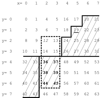
In this example, the range being queried (x = 2, ..., 3, y = 2, ..., 6) is indicated by the dotted rectangle. Its highest Z-value (MAX) is 45. In this example, the value F = 19 is encountered when searching a data structure in increasing Z-value direction, so we would have to search in the interval between F and MAX (hatched area). To speed up the search, one would calculate the next Z-value which is in the search range, called BIGMIN (36 in the example) and only search in the interval between BIGMIN and MAX (bold values), thus skipping most of the hatched area. Searching in decreasing direction is analogous with LITMAX which is the highest Z-value in the query range lower than F. The BIGMIN problem has first been stated and its solution shown in Tropf and Herzog.[10]
An extensive explanation of the LITMAX/BIGMIN calculation algorithm, together with Pascal Source Code (3D, easy to adapt to nD) and hints on how to handle floating point data and possibly negative data, is provided 2021 by Tropf: Here, bit interleaving is not done explicitly; the data structure has just pointers to the original (unsorted) database records. With a general record comparison function (greater-less-equal, in the sense of z-value), complications with bit sequences length exceeding the computer word length are avoided, and the code can easily be adapted to any number of dimensions and any record key word length.
As the approach does not depend on the one dimensional data structure chosen, there is still free choice of structuring the data, so well known methods such as balanced trees can be used to cope with dynamic data, and keeping the tree balance when inserting or deleting takes O(log n) time. The method is also used in UB-trees (balanced),[11] with the name "GetNextZ-address" for BIGMIN.
The Free choice makes it easier to incorporate the method into existing databases. This is in contrast for example to R-trees where special considerations are necessary.
Applying the method hierarchically (according to the data structure at hand), optionally in both increasing and decreasing direction, yields highly efficient multidimensional range search which is important in both commercial and technical applications, e.g. as a procedure underlying nearest neighbour searches. Z-order is one of the few multidimensional access methods that has found its way into commercial database systems.[12] The method is used in various technical applications of different fields[13] and in commercial database systems.[14]
As long ago as 1966, G.M.Morton proposed Z-order for file sequencing of a static two dimensional geographical database. Areal data units are contained in one or a few quadratic frames represented by their sizes and lower right corner Z-values, the sizes complying with the Z-order hierarchy at the corner position. With high probability, changing to an adjacent frame is done with one or a few relatively small scanning steps.[3]
Related structures
As an alternative, the Hilbert curve has been suggested as it has a better order-preserving behaviour,[5] and, in fact, was used in an optimized index, the S2-geometry.[15]
Applications
Linear algebra
The Strassen algorithm for matrix multiplication is based on splitting the matrices in four blocks, and then recursively splitting each of these blocks in four smaller blocks, until the blocks are single elements (or more practically: until reaching matrices so small that the Moser–de Bruijn sequence trivial algorithm is faster). Arranging the matrix elements in Z-order then improves locality, and has the additional advantage (compared to row- or column-major ordering) that the subroutine for multiplying two blocks does not need to know the total size of the matrix, but only the size of the blocks and their location in memory. Effective use of Strassen multiplication with Z-order has been demonstrated, see Valsalam and Skjellum's 2002 paper.[16]
Buluç et al. present a sparse matrix data structure that Z-orders its non-zero elements to enable parallel matrix-vector multiplication.[17]
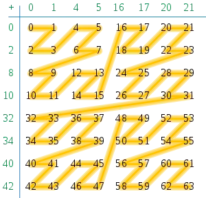
Matrices in linear algebra can also be traversed using a space-filling curve.[18] Conventional loops traverse a matrix row by row. Traversing with the Z-curve allows efficient access to the memory hierarchy.[19]
Texture mapping
Some GPUs store texture maps in Z-order to increase spatial locality of reference during texture mapped rasterization. This allows cache lines to represent rectangular tiles, increasing the probability that nearby accesses are in the cache. At a larger scale, it also decreases the probability of costly, so called, "page breaks" (i.e., the cost of changing rows) in SDRAM/DDRAM. This is important because 3D rendering involves arbitrary transformations (rotations, scaling, perspective, and distortion by animated surfaces).
These formats are often referred to as swizzled textures or twiddled textures. Other tiled formats may also be used.
n-body problem
The Barnes–Hut algorithm requires construction of an octree. Storing the data as a pointer-based tree requires many sequential pointer dereferences to iterate over the octree in depth-first order (expensive on a distributed-memory machine). Instead, if one stores the data in a hashtable, using octree hashing, the Z-order curve naturally iterates the octree in depth-first order.[5]
See also
References
- Discrete Global Grid Systems Abstract Specification (PDF), Open Geospatial Consortium, 2017
- Dugundji, James (1989), Wm. C. Brown (ed.), Topology, Dubuque (Iowa), p. 105, ISBN 0-697-06889-7
- Morton, G. M. (1966), A computer Oriented Geodetic Data Base; and a New Technique in File Sequencing (PDF), Technical Report, Ottawa, Canada: IBM Ltd.
- Bern, M.; Eppstein, D.; Teng, S.-H. (1999), "Parallel construction of quadtrees and quality triangulations", Int. J. Comput. Geom. Appl., 9 (6): 517–532, CiteSeerX 10.1.1.33.4634, doi:10.1142/S0218195999000303.
- Warren, M. S.; Salmon, J. K. (1993), "A parallel hashed Oct-Tree N-body algorithm", Proceedings of the 1993 ACM/IEEE conference on Supercomputing - Supercomputing '93, Portland, Oregon, United States: ACM Press, pp. 12–21, doi:10.1145/169627.169640, ISBN 978-0-8186-4340-8, S2CID 7583522
- Gargantini, I. (1982), "An effective way to represent quadtrees", Communications of the ACM, 25 (12): 905–910, doi:10.1145/358728.358741, S2CID 14988647.
- Chan, T. (2002), "Closest-point problems simplified on the RAM", ACM-SIAM Symposium on Discrete Algorithms.
- Connor, M.; Kumar, P (2009), "Fast construction of k-nearest neighbour graphs for point clouds", IEEE Transactions on Visualization and Computer Graphics (PDF)
- Har-Peled, S. (2010), Data structures for geometric approximation (PDF)
- Tropf, H.; Herzog, H. (1981), "Multidimensional Range Search in Dynamically Balanced Trees" (PDF), Angewandte Informatik, 2: 71–77.
- Ramsak, Frank; Markl, Volker; Fenk, Robert; Zirkel, Martin; Elhardt, Klaus; Bayer, Rudolf (2000), "Integrating the UB-tree into a Database System Kernel", Int. Conf. on Very Large Databases (VLDB) (PDF), pp. 263–272, archived from the original (PDF) on 2016-03-04
- https://dl.acm.org/doi/pdf/10.1145/280277.280279 Volker Gaede, Oliver Günther: Multidimensional access methods. ACM Computing Surveys volume=30 issue=2 pages=170–231 1998.
- Annotated list of research papers to technical applications using z-order range search (PDF)
- Annotated list of research papers to databases using z-order range search (PDF)
- S2 Geometry
- Vinod Valsalam, Anthony Skjellum: A framework for high-performance matrix multiplication based on hierarchical abstractions, algorithms and optimized low-level kernels. Concurrency and Computation: Practice and Experience 14(10): 805-839 (2002)
- Buluç, Aydın; Fineman, Jeremy T.; Frigo, Matteo; Gilbert, John R.; Leiserson, Charles E. (2009), "Parallel sparse matrix-vector and matrix-transpose-vector multiplication using compressed sparse blocks", ACM Symp. on Parallelism in Algorithms and Architectures (PDF), CiteSeerX 10.1.1.211.5256
- Martin Perdacher: Space-filling curves for improved cache-locality in shared memory environments. PhD thesis, University of Vienna 2020
- Martin Perdacher, Claudia Plant, Christian Böhm: Improved Data Locality Using Morton-order Curve on the Example of LU Decomposition. IEEE BigData 2020: pp. 351–360
External links
- STANN: A library for approximate nearest neighbor search, using Z-order curve
- Methods for programming bit interleaving, Sean Eron Anderson, Stanford University