Latin hypercube sampling
Latin hypercube sampling (LHS) is a statistical method for generating a near-random sample of parameter values from a multidimensional distribution. The sampling method is often used to construct computer experiments or for Monte Carlo integration.
LHS was described by Michael McKay of Los Alamos National Laboratory in 1979.[1] An independently equivalent technique was proposed by Vilnis Eglājs in 1977.[2] It was further elaborated by Ronald L. Iman and coauthors in 1981.[3] Detailed computer codes and manuals were later published.[4]
In the context of statistical sampling, a square grid containing sample positions is a Latin square if (and only if) there is only one sample in each row and each column. A Latin hypercube is the generalisation of this concept to an arbitrary number of dimensions, whereby each sample is the only one in each axis-aligned hyperplane containing it.
When sampling a function of variables, the range of each variable is divided into equally probable intervals. sample points are then placed to satisfy the Latin hypercube requirements; this forces the number of divisions, , to be equal for each variable. This sampling scheme does not require more samples for more dimensions (variables); this independence is one of the main advantages of this sampling scheme. Another advantage is that random samples can be taken one at a time, remembering which samples were taken so far.

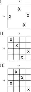
In two dimensions the difference between random sampling, Latin hypercube sampling, and orthogonal sampling can be explained as follows:
- In random sampling new sample points are generated without taking into account the previously generated sample points. One does not necessarily need to know beforehand how many sample points are needed.
- In Latin hypercube sampling one must first decide how many sample points to use and for each sample point remember in which row and column the sample point was taken. Such configuration is similar to having N rooks on a chess board without threatening each other.
- In orthogonal sampling, the sample space is divided into equally probable subspaces. All sample points are then chosen simultaneously making sure that the total set of sample points is a Latin hypercube sample and that each subspace is sampled with the same density.
Thus, orthogonal sampling ensures that the set of random numbers is a very good representative of the real variability, LHS ensures that the set of random numbers is representative of the real variability whereas traditional random sampling (sometimes called brute force) is just a set of random numbers without any guarantees.
References
- McKay, M.D.; Beckman, R.J.; Conover, W.J. (May 1979). "A Comparison of Three Methods for Selecting Values of Input Variables in the Analysis of Output from a Computer Code". Technometrics. American Statistical Association. 21 (2): 239–245. doi:10.2307/1268522. ISSN 0040-1706. JSTOR 1268522. OSTI 5236110.
- Eglajs, V.; Audze P. (1977). "New approach to the design of multifactor experiments". Problems of Dynamics and Strengths. 35 (in Russian). Riga: Zinatne Publishing House: 104–107.
- Iman, R.L.; Helton, J.C.; Campbell, J.E. (1981). "An approach to sensitivity analysis of computer models, Part 1. Introduction, input variable selection and preliminary variable assessment". Journal of Quality Technology. 13 (3): 174–183. doi:10.1080/00224065.1981.11978748.
- Iman, R.L.; Davenport, J.M.; Zeigler, D.K. (1980). Latin hypercube sampling (program user's guide). OSTI 5571631.
Further reading
- Tang, B. (1993). "Orthogonal Array-Based Latin Hypercubes". Journal of the American Statistical Association. 88 (424): 1392–1397. doi:10.2307/2291282. JSTOR 2291282.
- Owen, A.B. (1992). "Orthogonal arrays for computer experiments, integration and visualization". Statistica Sinica. 2: 439–452.
- Ye, K.Q. (1998). "Orthogonal column Latin hypercubes and their application in computer experiments". Journal of the American Statistical Association. 93 (444): 1430–1439. doi:10.2307/2670057. JSTOR 2670057.