Kinetic logic
Kinetic logic, developed by René Thomas, is a Qualitative Modeling approach feasible to model impact, feedback, and the temporal evolution of the variables. It uses symbolic descriptions and avoids continuous descriptions e.g. differential equations.The derivation of the dynamics from the interaction graphs of systems is not easy. A lot of parameters have to be inferred, for differential description, even if the type of each interaction is known in the graph. Even small modifications in parameters can lead to a strong change in the dynamics. Kinetic Logic is used to build discrete models, in which such details of the systems are not required. The information required can be derived directly from the graph of interactions or from a sufficiently explicit verbal description. It only considers the thresholds of the elements and uses logical equations to construct state tables. Through this procedure, it is a straightforward matter to determine the behavior of the system.[1]
Formalism


Following is René Thomas’s formalism for Kinetic Logic :
In a directed graph G = (V, A), we note G− (v) and G+ (v) the set of predecessors and successors of a node v ∈ V respectively.
Definition 1: A biological regulatory network (BRN) is a tuple G = (V, A, l, s, t, K) where
(V, A) is a directed graph denoted by G,
l is a function from V to N,
s is a function from A to {+, −},
t is a function from A to N such that, for all u ∈ V, if G+(u) is not empty then {t(u, v) | v ∈ G+(u)} = { 1, . . . , l(u)}.
K = {Kv | v ∈ V} is a set of maps: for each v ∈ V, Kv is a function from 2G− (v) to {0, . . . , l(v)} such that Kv(ω) ≤ Kv(ω_) for all ω ⊆ ω_ ⊆ G−(v).
The map l describes the domain of each variable v: if l (v) = k, the abstract concentration on v holds its value in {0, 1, . . . , k}. Similarly, the map s represents the sign of the regulation (+ for an activation, − for an inhibition). t (u, v) is the threshold of the regulation from u to v: this regulation takes place iff the abstract concentration of u is above t(u, v), in such a case the regulation is said active. The condition on these thresholds states that each variation of the level of u induces a modification of the set of active regulations starting from u. For all x ∈ [0, . . ., l(u) − 1], the set of active regulations of u, when the discrete expression level of u is x, differs from the set when the discrete expression level is x + 1. Finally, the map Kv allows us to define what is the effect of a set of regulators on the specific target v. If this set is ω ⊆ G− (v), then, the target v is subject to a set of regulations which makes it to evolve towards a particular level Kv(ω).
Definition 2 (States):
A state μ of a BRN G = (V, A, l, s, t, K) is a function from V to N such that μ (v) ∈ {0 .., l (v)} for all variables v ∈ V. We denote EG the set of states of G.
When μ (u) ≥ t (u, v) and s (u, v) = +, we say that u is a resource of v since the activation takes place. Similarly when μ (u) < t (u, v) and s (u, v) = −, u is also a resource of v since the inhibition does not take place (the absence of the inhibition is treated as an activation).
Definition 3 (Resource function):
Let G = (V, A, l, s, t, K) be a BRN. For each v ∈ V we define the resource function ωv: EG → 2G− (v) by:
ωv (μ) = {u ∈ G−(v) | (μ(u) ≥ t(u, v) and s(u, v) = +) or (μ (u) < t (u, v) and s (u, v) = −)}.
As said before, at state μ, Kv (ωv(μ)) gives the level towards which the variable v tends to evolve. We consider three cases,
- if μ(v) < Kv(ωv(μ)) then v can increase by one unit
- if μ(v) > Kv(ωv(μ)) then v can decrease by one unit
- if μ(v) = Kv (ωv (μ)) then v cannot evolve.
Definition 4 (Signs of derivatives):
Let G = (V, A, l, s, t, K) be a BRN and v ∈ V.
We define αv: EG → {+1, 0, −1} by αv(μ) =
+1 if Kv (ωv(μ)) > μ(u)
0 if Kv (ωv(μ)) = μ(u)
−1 if Kv (ωv(μ)) < μ(u)
The signs of derivatives show the tendency of the solution trajectories.
The state graph of BRN represents the set of the states that a BRN can adopt with transitions among them deduced from the previous rules:
Definition 5 (State graph):
Let G = (V, A, b, s, t,K) be a BRN. The state graph of G is a directed graph G = (EG, T) with (μ, μ_) ∈ T if there exists v ∈ V such that:
αv (μ) ≠ 0 and μ’ (v) = μ (v) + αv (μ) and μ (u) = μ’ (u), ∀u ∈ V \ {v}.[2]
Critical Assumptions
The critical assumptions of Kinetic Logic are:
- The elements of system have slight effect on each other until they reach a threshold.
- At high levels the effect on each other tends to reach a plateau. So an element is present when greater than the threshold level and absent when it is below the threshold level.[3]
Steps of Application
Following are the steps of Application of Kinetic Logic (Also shown in figure A).[4]
Biological Regulatory Network (BRN)
Keeping the research problem in mind, the behavior of elements in the system and their interactions are studied. Elements of a system can interact positively or negatively, that is, the level of an element may activate or reduce the rate of production of other elements or of itself. These interactions are represented as positive (activation) or negative (inhibition).
When elements are connected in a topologically circular way, they exert an influence on their own rate of synthesis and they form a feedback loop. A feedback loop is positive or negative according to whether it contains an even or odd number of negative interactions. In a positive loop, each element of the system exerts a positive effect on its own rate of synthesis, whereas in a simple negative loop, each element has a negative effect on its own rate of synthesis. A simple positive feedback loop results in epigenetic regulation and have multiple steady states and a simple negative feedback loop results in homeostatic regulation.
Abstraction: A chain of positive interactions is equivalent to a direct positive interaction between the two extreme elements, and any two negative interactions cancel out each other’s effect. In this way, any simple feedback loop can be abridged to a one-element loop, positive or negative according to the number of negative interactions (even or odd) in the original loop. Accordingly, through extensive literature survey and the application of the above-mentioned rules, a BRN is abstracted.
Logical Variable and Functions
Logical variables are associated with the elements of the system to describe the state of the system. They consist of the logical values. For example, a system whose state is appropriately described by the levels of substances a, b, and c, each of which can be absent, present at low level, or present at high level are represented by logical values 0, 1, and 2 respectively.
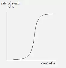
If a product an acts to stimulate the production of b, it is a positive regulator. In this case, the rate of synthesis of b increases with increasing concentration of a, and makes a curve similar to that shown in figure B.
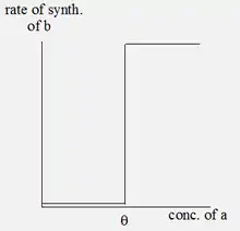
There is little effect of a, until it reaches a threshold concentration theta, and at higher concentrations a plateau is reached which shows the maximal rate of synthesis of b. Such a nonlinear, bounded curve is called a sigmoid. It can be suggested that a is "absent" for a < theta and "present" for a > theta. The sigmoid curve can be approximated by the step function, as in figure C.
Not only logical variables (x, y, z ...) are associated to the elements, that represent their level (e.g., concentration), but also logical functions (X, Y, Z ...) whose value reflects the rate of synthesis of the element. Thus,
x = 0 means "gene product absent"
x = 1 means "gene product present"
&
X = 0 means "gene off"
X = 1 means "gene on"
Graph of Interactions and Logical Equations
Kinetic Logic has two forms depending on the following two types of descriptions:
Naïve Logical Description
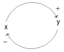
Consider a simple two-element system in which product x activates gene Y and product y represses gene X as shown in figure D. Each variable takes only two values; 0 and 1. In other words,
X = 1 if y = 0 (X "on” if y absent)
Y = 1 if x = 1 (Y "on" if x present)
The logical relation of the system can be written:
X =y
Y=x
Generalized Kinetic Logic
The naive logical description can be generalized and made to accommodate situations in which some variables take more than two values, without complicating the analysis. Any variable has a number of biologically relevant levels, determined by the number of elements regulated by the product x. There is a specific threshold for each regulatory interaction, so if x regulates n elements, it will have up to n different thresholds.
For the logical sum, there is a procedure that assigns a specific weight to each term in the logical relation. According to the scale of thresholds of the corresponding variable, the weighted algebraic sum is then discretized, so an n-valued variable is associated with an n-valued function. After discretization the integers of certain weights or sums of weights are called logical parameters.
Generalized Kinetic Logic, although maintaining the analytic simplicity of the naive description, has certain features in common with the differential description. The generalized logical relations are completely independent of the differential description and can be directly derived from the graph of interactions or from an explicit verbal description.
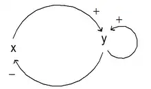
Consider an example of two elements in figure E. Using a software, this graph of interactions is drawn as shown in figure F. There are two thresholds assigned to element y: Ѳ12, concerning its interaction with x and Ѳ22, concerning its interaction with itself. The variable y and function Y have three possible values: 0, 1, and 2. Element x have a single threshold, Ѳ21, because of the interaction x to +y, so the variable x and function X will be two-valued.
State Table and State Graph
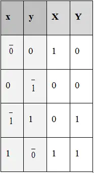
The state table of graph of interactions in figure D is shown in figure G. This table states for each state of the variables (x, y) i.e. present or absent, which products are synthesized and which are not synthesized at a significant rate. Consider the state 00/10, in which both of the gene products are absent but gene X is on. As product x is absent but being synthesized so it can be expected that in near future it will be present and the logical value of x will change from 0 to 1. This can be described by the notation Ō, in which the dash above the digit is due to the fact that variable x is committed to change its value from 0 to 1. Generally, a dash over the figure representing the logical value of a variable each time this value is different from that of the corresponding function. The state just considered can thus be represented as ŌO.
Time Delays
The movement of a system from one state to another depends on the time delays. The time delays in systems are short time shifts of arbitrary duration. In view of the relation between a function (gene on or off) and its associated variable (gene product present or absent), the time delays become real entities whose values, far from being arbitrary, reflect specific physical processes (synthesis, degradation, dilution, etc.). The values of the different time delays play an important role in determining the pathway along which the system evolves.
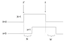
The temporal relation between a logical variable x which is associated with the level of an element and a logical function X which is associated with its evolution can be explained as follows.
Consider a gene that is off (X = 0) for a considerable time, then is switched on (X = 1) by a signal, and then, after some time, it is switched off again (X= 0) by another signal and the product reappears but not immediately until a proper delay tx has elapsed. If a signal switches the gene off temporarily, the product is still present because it also requires a time delay tx’. This can be represented graphically as shown in figure H. Using the state table the temporal sequence of states of the system can be represented as shown in figure I.
Identifying Cycles and Stable Steady States
Cycles
The state table in D can be used to identify the cyclic behavior of the system. We can see that state 01 changes to 00, and 00 changes to 10, 10 changes to 11 and 11 changes back to 01. This represents a cycle as the system starts from the state 01 and returns to the same state. The system keeps oscillating between these states.
Deadlocks
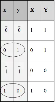
Consider another example in which:
X=y
Y=x
The state table for the system is shown in figure J. The states that are encircled are stable states, as they do not evolve towards any other state. The logical stable states are defined as those for which the vectors xy . .. and XY ... are equal. When we considered the time delays i.e. from ŌŌ the system will proceed to state 1 0 or to state 01, according to whether tx < ty or ty < tx, and from ĪĪ the system will proceed to state 10 or to state 0 1 according to whether ty < tx or tx < ty. The state graph representing delays is shown in figure K.
The sequence of states a system depends on the relative values of the time delays. It is assumed that two delays (or sums of delays) are never exactly equal, therefore that two variables will not change their values at the same instant. But do not exclude the possibility because if this rule is applied rigidly, it could occasionally lead to the loss of interesting pathways.
Analyzing the Results
The cycles and the deadlock states identified by this process are then analyzed by comparing them with the invitro and invivo findings. These results can be used to make important predictions about the system. Cyclic behaviors correspond to homeostatic regulations that retain the level of a variable at or near a fixed or optimal value. Deadlocks represent epigenetic regulation in which the concentrations exist between extreme levels.[5]
History
The first approach for qualitative modeling was based on extreme discretization since all genes could be either on (present) or off (absent).[6] This Boolean approach was generalized into a multi-valued approach i.e. Kinetic Logic,[7][8] in which logical identification of all steady states became possible.[9]
Application
Kinetic logic has been employed to study the factors that influence the selection of specific pathway from many different pathways that the system can follow and the factors that lead the system towards stable states and cyclic behaviors. It has been used to reveal the logic that lie behind the functional organization and kinetic behavior of molecules. Model checking techniques have also been applied to models built through kinetic logic, in order to infer their continuous behaviors.[10]
Kinetic logic has been applied on many different types of systems in biology, Psychology and Psychiatry.[11] Mostly Kinetic Logic has been used in modeling the biological networks especially the Gene Regulatory Networks (GRNs). Following are the examples in which Kinetic Logic was employed as the modeling formalism:
- To model the dynamics of chronic psychosis and schizophrenia.[12][13]
- To show that how residence time of the hormone on the receptor can decide the specificity of signaling between the alternative metabolic or mitogenic pathways,[14]
- To explain the positive (cell proliferation and cytokine production) and negative (anergy induction) signaling of T lymphocytes; to determine how the timing of the binding and intracellular signal-transduction events can influence the properties of receptor signaling and decide the type of cellular response[15]
- To demonstrate how prion infection proceeds[16]
- To model other biological regulatory networks (BRNs) like toy gene, lambda phage (Ahmad and Roux, 2008), Pseudomonas aeruginosa and circadian rhythm.[17]
- To reveal the logic that lie behind the functional organization and kinetic behavior of the thioredoxin system [18]
Tool
As theoretical analysis through Kinetic Logic is a time consuming process, a tool known as Genotech, for modeling and analysis of BRNs was developed on the basis of Kinetic Logic and has been used for a number of Kinetic Logic-based studies.[19] It analyzes behaviors like stable cycles, stable steady states and paths in the state graph (discrete model) of biological systems, accelerating the process of modeling.[20] GenoTech is extremely useful as it allows repeated experimentation by automating the whole process. This tool is available on request.
Books
- Thomas, René, ed. (1979). Kinetic logic: a Boolean approach to the analysis of complex regulatory systems. Lecture Notes in Biomathematics. Vol. 29. Springer-Verlag. ISBN 0-387-09556-X. OCLC 5447473.
- Thomas, René; D'Ari, Richard (1990). Biological feedback. CRC Press. ISBN 0-8493-6766-2. OCLC 20357419.
References
- Thomas R., (1973) Boolean formulization of genetic control circuits. Journal of Theoretical Biology. 42 (3): 565–583.
- Thomas R., (1978) Logical analysis of systems comprising feedback loops. J Theor Biol.73(4): 631–656.
- Kupper Z and Hoffmann H., (1995) Modeling the Dynamics of Psychosis by Kinetic Logic (4-95). Bern, Switzerland: University of Bern, Department of Social and Community Psychiatry.
- Thomas R., and D’Ari R., (1990) Biological feedback. FL: CRC Press, Boca Raton.
- Thomas R., and D’Ari R., (1990) Biological feedback. FL: CRC Press, Boca Raton.
- Thomas R., (1978) Logical analysis of systems comprising feedback loops. J Theor Biol.73(4): 631–656.
- Thomas R., (1991) Regulatory networks seen as asynchronous automata: a logical description. J Theor Biol. 153: 1–23.
- Snoussi E., (1989) Qualitative dynamics of a piecewise-linear differential equations: a discrete mapping approach. DSS. 4:189–207.
- Snoussi E., and Thomas R., (1993) Logical identification of all steady states : the concept of feedback loop characteristic states. Bull Math Biol. 55(5):973–991.
- J. Ahmad, and O. Roux, “Analysing formal models of genetic regulatory networks with delays,” Int. J. Bioinformatics Research and Applications. vol. 4. pp. 240-262, 2008.
- Kupper Z and Hoffman H., (1995) Modeling the Dynamics of Psychosis by Kinetic Logic (4-95). Bern, Switzerland: University of Bern, Department of Social and Community Psychiatry.
- Kupper Z and Hoffman H., (1995) Modeling the Dynamics of Psychosis by Kinetic Logic (4-95). Bern, Switzerland: University of Bern, Department of Social and Community Psychiatry.
- Breedlove S.M., Rosenzweig M.R., and Watson N.V., (2010) Biological Psychology (6th Edition): ISBN 0878933247
- de Jong H., (2002) Modeling and simulation of genetic regulatory systems: a literature review. J Comput Biol. 9(1):67–103.
- de Jong H., (2002) Modeling and simulation of genetic regulatory systems: a literature review. J Comput Biol. 9(1):67–103.
- de Jong H., (2002) Modeling and simulation of genetic regulatory systems: a literature review. J Comput Biol. 9(1):67–103.
- J. Ahmad, and O. Roux, “Analysing formal models of genetic regulatory networks with delays,” Int. J. Bioinformatics Research and Applications. vol. 4. pp. 240-262, 2008.
- de Jong H., (2002) Modeling and simulation of genetic regulatory systems: a literature review. J Comput Biol. 9(1):67–103.
- J. Ahmad, “Modélisation hybride et analyse des dynamiques des réseaux de régulations biologiques en tenant compte des délais, “ PhD thesis, Ecole Centrale de Nantes, France, 2009.
- Thomas R., and D’Ari R., (1990) Biological feedback. FL: CRC Press, Boca Raton.