Population dynamics of fisheries

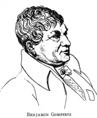
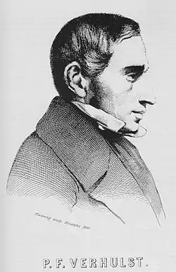
The first principle of population dynamics is widely regarded as the exponential law of Malthus, as modelled by the Malthusian growth model. The early period was dominated by demographic studies such as the work of Benjamin Gompertz and Pierre François Verhulst in the early 19th century, who refined and adjusted the Malthusian demographic model. A more general model formulation was proposed by F.J. Richards in 1959, by which the models of Gompertz, Verhulst and also Ludwig von Bertalanffy are covered as special cases of the general formulation.[6]

The population size (usually denoted by N) is the number of individual organisms in a population.

The effective population size (N_e) was defined by Sewall Wright, who wrote two landmark papers on it (Wright 1931, 1938). He defined it as "the number of breeding individuals in an idealized population that would show the same amount of dispersion of allele frequencies under random genetic drift or the same amount of inbreeding as the population under consideration". It is a basic parameter in many models in population genetics. N_e is usually less than N (the absolute population size).

Small population size results in increased genetic drift. Population bottlenecks are when population size reduces for a short period of time.

Overpopulation may indicate any case in which the population of any species of animal may exceed the carrying capacity of its ecological niche.

Virtual population analysis (VPA) is a cohort modeling technique commonly used in fisheries science for reconstructing historical fish numbers at age using information on death of individuals each year. This death is usually partitioned into catch by fisheries and natural mortality. VPA is virtual in the sense that the population size is not observed or measured directly but is inferred or back-calculated to have been a certain size in the past in order to support the observed fish catches and an assumed death rate owing to non-fishery related causes.

The minimum viable population (MVP) is a lower bound on the population of a species, such that it can survive in the wild. More specifically MVP is the smallest possible size at which a biological population can exist without facing extinction from natural disasters or demographic, environmental, or genetic stochasticity.[7] The term "population" refers to the population of a species in the wild.

As a reference standard, MVP is usually given with a population survival probability of somewhere between ninety and ninety-five percent and calculated for between one hundred and one thousand years into the future.

The MVP can be calculated using computer simulations known as population viability analyses (PVA), where populations are modelled and future population dynamics are projected.

In population ecology and economics, the maximum sustainable yield or MSY is, theoretically, the largest catch that can be taken from a fishery stock over an indefinite period.[8][9] Under the assumption of logistic growth, the MSY will be exactly at half the carrying capacity of a species, as this is the stage at when population growth is highest. The maximum sustainable yield is usually higher than the optimum sustainable yield.

This logistic model of growth is produced by a population introduced to a new habitat or with very poor numbers going through a lag phase of slow growth at first. Once it reaches a foothold population it will go through a rapid growth rate that will start to level off once the species approaches carrying capacity. The idea of maximum sustained yield is to decrease population density to the point of highest growth rate possible. This changes the number of the population, but the new number can be maintained indefinitely, ideally.

MSY is extensively used for fisheries management.[10][11] Unlike the logistic (Schaefer) model, MSY in most modern fisheries models occurs at around 30-40% of the unexploited population size.[12] This fraction differs among populations depending on the life history of the species and the age-specific selectivity of the fishing method.

However, the approach has been widely criticized as ignoring several key factors involved in fisheries management and has led to the devastating collapse of many fisheries. As a simple calculation, it ignores the size and age of the animal being taken, its reproductive status, and it focuses solely on the species in question, ignoring the damage to the ecosystem caused by the designated level of exploitation and the issue of bycatch. Among conservation biologists it is widely regarded as dangerous and misused.[4][5]

Recruitment is the number of new young fish that enter a population in a given year. The size of fish populations can fluctuate by orders of magnitude over time, and five to 10-fold variations in abundance are usual. This variability applies across time spans ranging from a year to hundreds of years. Year to year fluctuations in the abundance of short lived forage fish can be nearly as great as the fluctuations that occur over decades or centuries. This suggests that fluctuations in reproductive and recruitment success are prime factors behind fluctuations in abundance. Annual fluctuations often seem random, and recruitment success often has a poor relationship to adult stock levels and fishing effort. This makes prediction difficult.[13]

The recruitment problem is the problem of predicting the number of fish larvae in one season that will survive and become juvenile fish in the next season. It has been called "the central problem of fish population dynamics"[14] and “the major problem in fisheries science".[15] Fish produce huge volumes of larvae, but the volumes are very variable and mortality is high. This makes good predictions difficult.[16]

According to Daniel Pauly,[15][17] the definitive study was made in 1999 by Ransom Myers.[18] Myers solved the problem "by assembling a large base of stock data and developing a complex mathematical model to sort it out. Out of that came the conclusion that a female in general produced three to five recruits per year for most fish.”[15]

Fishing effort is a measure of the anthropogenic work input used to catch fish. A good measure of the fishing effort will be approximately proportional to the amount of fish captured. Different measures are appropriate for different kinds of fisheries. For example, the fishing effort exerted by a fishing fleet in a trawl fishery might be measured by summing the products of the engine power for each boat and time it spent at sea (KW × days). For a gill-net fishery the effort might be measured by summing the products of the length of each set net and the time it was set in the water (Km × soak time). In fisheries where boats spend a lot of time looking for fish, a measure based on search time may be used.[19][20][21]

The Traffic Light colour convention, showing the concept of Harvest Control Rule (HCR), specifying when a rebuilding plan is mandatory in terms of precautionary and limit reference points for spawning biomass and fishing mortality rate.

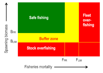
The notion of overfishing hinges on what is meant by an acceptable level of fishing.

A current operational model used by some fisheries for predicting acceptable levels is the Harvest Control Rule (HCR). This formalizes and summarizes a management strategy which can actively adapt to subsequent feedback. The HCR is a variable over which the management has some direct control and describes how the harvest is intended to be controlled by management in relation to the state of some indicator of stock status. For example, a harvest control rule can describe the various values of fishing mortality which will be aimed at for various values of the stock abundance. Constant catch and constant fishing mortality are two types of simple harvest control rules.[22]

• Biological overfishing occurs when fishing mortality has reached a level where the stock biomass has negative marginal growth (slowing down biomass growth), as indicated by the red area in the figure. Fish are being taken out of the water so quickly that the replenishment of stock by breeding slows down. If the replenishment continues to slow down for long enough, replenishment will go into reverse and the population will decrease.
• Economic or bioeconomic overfishing additionally considers the cost of fishing and defines overfishing as a situation of negative marginal growth of resource rent. Fish are being taken out of the water so quickly that the growth in the profitability of fishing slows down. If this continues for long enough, profitability will decrease.

A metapopulation is a group of spatially separated populations of the same species which interact at some level. The term was coined by Richard Levins in 1969. The idea has been most broadly applied to species in naturally or artificially fragmented habitats. In Levins' own words, it consists of "a population of populations".[23]

A metapopulation generally consists of several distinct populations together with areas of suitable habitat which are currently unoccupied. Each population cycles in relative independence of the other populations and eventually goes extinct as a consequence of demographic stochasticity (fluctuations in population size due to random demographic events); the smaller the population, the more prone it is to extinction.

Although individual populations have finite life-spans, the population as a whole is often stable because immigrants from one population (which may, for example, be experiencing a population boom) are likely to re-colonize habitat which has been left open by the extinction of another population. They may also emigrate to a small population and rescue that population from extinction (called the rescue effect).

• 
  Malthus
• 
  Gompertz
• 
  Verhulst

Age can be determined by counting growth rings in fish scales, otoliths, cross-sections of fin spines for species with thick spines such as triggerfish, or teeth for a few species. Each method has its merits and drawbacks. Fish scales are easiest to obtain, but may be unreliable if scales have fallen off of the fish and new ones grown in their places. Fin spines may be unreliable for the same reason, and most fish do not have spines of sufficient thickness for clear rings to be visible. Otoliths will have stayed with the fish throughout its life history, but obtaining them requires killing the fish. Also, otoliths often require more preparation before ageing can occur.

An age class structure with gaps in it, for instance a regular bell curve for the population of 1-5 year-old fish, excepting a very low population for the 3-year-olds, implies a bad spawning year 3 years ago in that species.

Often fish in younger age class structures have very low numbers because they were small enough to slip through the sampling nets, and may in fact have a very healthy population.

A population cycle occurs where populations rise and fall over a predictable period of time. There are some species where population numbers have reasonably predictable patterns of change although the full reasons for population cycles is one of the major unsolved ecological problems. There are a number of factors which influence population change such as availability of food, predators, diseases and climate.

Trophic cascades occur when predators in a food chain suppress the abundance of their prey, thereby releasing the next lower trophic level from predation (or herbivory if the intermediate trophic level is an herbivore). For example, if the abundance of large piscivorous fish is increased in a lake, the abundance of their prey, zooplanktivorous fish, should decrease, large zooplankton abundance should increase, and phytoplankton biomass should decrease. This theory has stimulated new research in many areas of ecology. Trophic cascades may also be important for understanding the effects of removing top predators from food webs, as humans have done in many places through hunting and fishing activities.

Classic examples

1. In lakes, piscivorous fish can dramatically reduce populations of zooplanktivorous fish, zooplanktivorous fish can dramatically alter freshwater zooplankton communities, and zooplankton grazing can in turn have large impacts on phytoplankton communities. Removal of piscivorous fish can change lake water from clear to green by allowing phytoplankton to flourish.[24]
2. In the Eel River, in Northern California, fish (steelhead and roach) consume fish larvae and predatory insects. These smaller predators prey on midge larvae, which feed on algae. Removal of the larger fish increases the abundance of algae.[25]
3. In Pacific kelp forests, sea otters feed on sea urchins. In areas where sea otters have been hunted to extinction, sea urchins increase in abundance and decimate kelp[26]

A recent theory, the mesopredator release hypothesis, states that the decline of top predators in an ecosystem results in increased populations of medium-sized predators (mesopredators).

• The classic population equilibrium model is Verhulst's 1838 growth model:

${\displaystyle {\frac {dN}{dt}}=rN\left(1-{\frac {N}{K}}\right)}$

where N(t) represents number of individuals at time t, r the intrinsic growth rate and K is the carrying capacity, or the maximum number of individuals that the environment can support.

• The individual growth model, published by von Bertalanffy in 1934, can be used to model the rate at which fish grow. It exists in a number of versions, but in its simplest form it is expressed as a differential equation of length (L) over time (t):

${\displaystyle L'(t)=r_{B}\left(L_{\infty }-L(t)\right)}$

where r_B is the von Bertalanffy growth rate and L_∞ the ultimate length of the individual.

• Schaefer published a fishery equilibrium model based on the Verhulst model with an assumption of a bi-linear catch equation, often referred to as the Schaefer short-term catch equation:

${\displaystyle H(E,X)=qEX\!}$

where the variables are; H, referring to catch (harvest) over a given period of time (e.g. a year); E, the fishing effort over the given period; X, the fish stock biomass at the beginning of the period (or the average biomass), and the parameter q represents the catchability of the stock.

Assuming the catch to equal the net natural growth in the population over the same period (${\displaystyle {\dot {X}}=0}$), the equilibrium catch is a function of the long term fishing effort E:

${\displaystyle H(E)=qKE(1-{\frac {qE}{r}})}$

r and K being biological parameters representing intrinsic growth rate and natural equilibrium biomass respectively.

• The Baranov catch equation of 1918 is perhaps the most used equation in fisheries modelling.[27] It gives the catch in numbers as a function of initial population abundance N₀ and fishing F and natural mortality M:

${\displaystyle C={\frac {F}{F+M}}(1-e^{-(F+M)T})N_{0}}$

where T is the time period and is usually left out (i.e. T=1 is assumed). The equation assumes that fishing and natural mortality occur simultaneously and thus "compete" with each other. The first term expresses the proportion of deaths that are caused by fishing, and the second and third term the total number of deaths.[28]

• The Ricker model is a classic discrete population model which gives the expected number (or density) of individuals N_t + 1 in generation t + 1 as a function of the number of individuals in the previous generation,

${\displaystyle N_{t+1}=N_{t}e^{r(1-{\frac {N_{t}}{k}})}}$

Here r is interpreted as an intrinsic growth rate and k as the carrying capacity of the environment. The Ricker model was introduced in the context of the fisheries by Ricker (1954).[29]

• The Beverton–Holt model, introduced in the context of fisheries in 1957, is a classic discrete-time population model which gives the expected number n _t+1 (or density) of individuals in generation t + 1 as a function of the number of individuals in the previous generation,

${\displaystyle n_{t+1}={\frac {R_{0}n_{t}}{1+n_{t}/M}}.}$

Here R₀ is interpreted as the proliferation rate per generation and K = (R₀ − 1) M is the carrying capacity of the environment.

The classic predator–prey equations are a pair of first order, non-linear, differential equations used to describe the dynamics of biological systems in which two species interact, one a predator and one its prey. They were proposed independently by Alfred J. Lotka in 1925 and Vito Volterra in 1926.

An extension to these are the competitive Lotka–Volterra equations, which provide a simple model of the population dynamics of species competing for some common resource.

In the 1930s Alexander Nicholson and Victor Bailey developed a model to describe the population dynamics of a coupled predator–prey system. The model assumes that predators search for prey at random, and that both predators and prey are assumed to be distributed in a non-contiguous ("clumped") fashion in the environment.[30]

In the late 1980s, a credible, simple alternative to the Lotka–Volterra predator-prey model (and its common prey dependent generalizations) emerged, the ratio dependent or Arditi–Ginzburg model.[31] The two are the extremes of the spectrum of predator interference models. According to the authors of the alternative view, the data show that true interactions in nature are so far from the Lotka–Volterra extreme on the interference spectrum that the model can simply be discounted as wrong. They are much closer to the ratio dependent extreme, so if a simple model is needed one can use the Arditi-Ginzburg model as the first approximation.[32]

• Berryman, Alan (2002) Population Cycles. Oxford University Press US. ISBN 0-19-514098-2
• de Vries, Gerda; Hillen, Thomas; Lewis, Mark; Schonfisch, Birgitt and Muller, Johannes (2006) A Course in Mathematical Biology SIAM. ISBN 978-0-89871-612-2
• Haddon, Malcolm (2001) Modelling and quantitative methods in fisheries Chapman & Hall. ISBN 978-1-58488-177-3
• Hilborn, Ray and Walters, Carl J (1992) Quantitative Fisheries Stock Assessment Springer. ISBN 978-0-412-02271-5
• McCallum, Hamish (2000) Population Parameters Blackwell Publishing. ISBN 978-0-86542-740-2
• Prevost E and Chaput G (2001) Stock, recruitment and reference points Institute National de la Recherche Agronomique. ISBN 2-7380-0962-X.
• Plagányi, Éva, Models for an ecosystem approach to fisheries. FAO Fisheries Technical Paper. No. 477. Rome, FAO. 2007. 108p
• Quinn, Terrance J. II and Richard B. Deriso (1999) Quantitative Fish Dynamics.Oxford University Press ISBN 0-19-507631-1
• Sparre, Per and Hart, Paul J B (2002) Handbook of Fish Biology and Fisheries, Chapter13: Choosing the best model for fisheries assessment. Blackwell Publishing. ISBN 0-632-06482-X
• Turchin, P. 2003. Complex Population Dynamics: a Theoretical/Empirical Synthesis. Princeton, NJ: Princeton University Press.

References

- Wilderbuer, Thomas K.; Zhang, Chang Ik (1999). "Evaluation of the population dynamics and yield characteristics of Alaska plaice, Pleuronectes quadrituberculatus, in the eastern Bering Sea". Fisheries Research. 41 (2): 183–200. doi:10.1016/S0165-7836(99)00012-0.
- Zabel, Richard W.; et al. (2003). "Ecologically Sustainable Yield". American Scientist. 91 (2): 150–157. doi:10.1511/2003.2.150. JSTOR 27858183.
- Caswell, H. (2001). Matrix population models: Construction, analysis and interpretation (2nd ed.). Sunderland, Massachusetts: Sinauer Associates. ISBN 0-87893-096-5.
- Larkin, P. A. (1977). "An Epitaph for the Concept of Maximum Sustained Yield". Transactions of the American Fisheries Society. 106 (1): 1–11. doi:10.1577/1548-8659(1977)106<1:AEFTCO>2.0.CO;2.
- Walters, C.; Maguire, J. (1996). "Lessons for stock assessment from the northern cod collapse". Reviews in Fish Biology and Fisheries. 6 (2): 125–137. doi:10.1007/BF00182340. S2CID 20224324.
- Richards, F. J. (1959). "A Flexible Growth Function for Empirical Use". Journal of Experimental Botany. 10 (2): 290–301. doi:10.1093/jxb/10.2.290.
- Holsinger, Kent (2007). "Types of stochastic threats". Archived from the original on November 20, 2008. Retrieved 2007-11-04.
- European Union (2006). "Management based on maximum sustainable yield". Archived from the original on 2007-12-23.
- European Union (2006). "Questions and Answers on Maximum Sustainable Yield (MSY)".
- WWF Publications (2007). "The Maximum Sustainable Yield objective in Fisheries".
- New Zealand Ministry of Fisheries. "MSY Harvest Strategies".
- See e.g. Thorpe, Robert B.; et al. (2015). "Evaluation and management implications of uncertainty in a multispecies size-structured model of population and community responses to fishing". Methods in Ecology and Evolution. 6 (1): 49–58. doi:10.1111/2041-210X.12292. PMC 4390044. PMID 25866615.
- Houde, D. E. (2009). "Recruitment variability". In Jakobsen, T.; Fogarty, M. J.; Megrey, B. A.; Moksness, E. (eds.). Fish Reproductive Biology. Wiley-Blackwell. ISBN 978-1-4051-2126-2.
- Beyer, J. E. (1981). Aquatic ecosystems-an operational research approach. University of Washington Press. ISBN 0-295-95719-0.
- "Ransom A. Myers, 54, Dies; Expert on Loss of Fish Stocks". The New York Times. 29 March 2007.
- Bakun, A. (1985). "Comparative studies and the recruitment problem: Searching for generalizations" (PDF). CalCOFI Report. 26. Archived from the original (PDF) on 2008-12-01.
- Pauly, Daniel (10 May 2007). "Ransom Aldrich Myers (1952-2007)" (PDF). Nature. 447 (7141): 160. doi:10.1038/447160a. PMID 17495917. S2CID 4430142.
- Myers, R. A. (1995). "Recruitment of marine fish: the relative roles of density-dependent and density-independent mortality in the egg, larval, and juvenile stages" (PDF). Marine Ecology Progress Series. 128: 305–310. Archived from the original (PDF) on April 25, 2011.
- "Fishing effort". Glossary of Statistical Terms. Review of Fisheries in OECD Countries, 1998. 5 March 2003. Retrieved 21 April 2019.
- "Fishing effort". European Commission. Retrieved 21 April 2019.
- "Fishing effort measurement". Food and Agriculture Organization of the United Nations. Retrieved 21 April 2019.
- Coad, Brian W.; McAllister, Don E. (2008). "Dictionary of Ichthyology". Archived from the original on 20 July 2011. Retrieved 2 January 2015.
- Levins, R. (1969). "Some demographic and genetic consequences of environmental heterogeneity for biological control". Bulletin of the Entomological Society of America. 15 (3): 237–240. doi:10.1093/besa/15.3.237.
- Carpenter, S. R.; Kitchell, J. F.; Hodgson, J. R. (1985). "Cascading trophic interactions and lake productivity". BioScience. 35 (10): 634–639. doi:10.2307/1309989. JSTOR 1309989.
- Power, M. E. (1990). "Effects of fish in river food webs". Science. 250 (4982): 811–814. Bibcode:1990Sci...250..811P. doi:10.1126/science.250.4982.811. PMID 17759974. S2CID 24780727.
- Estes, J. A.; Palmisano, J. F. (1974). "Sea otters: their role in structuring nearshore communities". Science. 185 (4156): 1058–1060. Bibcode:1974Sci...185.1058E. doi:10.1126/science.185.4156.1058. PMID 17738247. S2CID 35892592.
- Quinn, Terrance J. II (2003). "Ruminations on the development and future of population dynamics models in fisheries". Natural Resource Modeling. 16 (4): 341–392. CiteSeerX 10.1.1.473.3765. doi:10.1111/j.1939-7445.2003.tb00119.x. S2CID 153420994.
- Baranov, F. I. (1918). "On the question of the biological basis of fisheries". Izvestiya. 1: 81–128. (Translated from Russian by W.E. Ricker, 1945)
- Ricker, WE (1954). Stock and recruitment. Journal of the Fisheries Research Board of Canada.
- Hopper, J. L. (1987). "Opportunities and Handicaps of Antipodean Scientists: A. J. Nicholson and V. A. Bailey on the Balance of Animal Populations". Historical Records of Australian Science. 7 (2): 179–188. doi:10.1071/HR9880720179.
- Arditi, R.; Ginzburg, L. R. (1989). "Coupling in predator-prey dynamics: ratio dependence". Journal of Theoretical Biology. 139 (3): 311–326. Bibcode:1989JThBi.139..311A. doi:10.1016/S0022-5193(89)80211-5.
- Arditi, R.; Ginzburg, L. R. (2012). How Species Interact: Altering the Standard View on Trophic Ecology. New York: Oxford University Press.
Further reading