Compartmental models in epidemiology
Compartmental models are a very general modelling technique. They are often applied to the mathematical modelling of infectious diseases. The population is assigned to compartments with labels – for example, S, I, or R, (Susceptible, Infectious, or Recovered). People may progress between compartments. The order of the labels usually shows the flow patterns between the compartments; for example SEIS means susceptible, exposed, infectious, then susceptible again.
The origin of such models is the early 20th century, with important works being that of Ross[1] in 1916, Ross and Hudson in 1917,[2][3] Kermack and McKendrick in 1927[4] and Kendall in 1956.[5] The Reed–Frost model was also a significant and widely-overlooked ancestor of modern epidemiological modelling approaches.[6]
The models are most often run with ordinary differential equations (which are deterministic), but can also be used with a stochastic (random) framework, which is more realistic but much more complicated to analyze.
Models try to predict things such as how a disease spreads, or the total number infected, or the duration of an epidemic, and to estimate various epidemiological parameters such as the reproductive number. Such models can show how different public health interventions may affect the outcome of the epidemic, e.g., what the most efficient technique is for issuing a limited number of vaccines in a given population.
The SIR model
The SIR model[7][8][9][10] is one of the simplest compartmental models, and many models are derivatives of this basic form. The model consists of three compartments:
- S: The number of susceptible individuals. When a susceptible and an infectious individual come into "infectious contact", the susceptible individual contracts the disease and transitions to the infectious compartment.
- I: The number of infectious individuals. These are individuals who have been infected and are capable of infecting susceptible individuals.
- R for the number of removed (and immune) or deceased individuals. These are individuals who have been infected and have either recovered from the disease and entered the removed compartment, or died. It is assumed that the number of deaths is negligible with respect to the total population. This compartment may also be called "recovered" or "resistant".
This model is reasonably predictive[11] for infectious diseases that are transmitted from human to human, and where recovery confers lasting resistance, such as measles, mumps and rubella. It has also been used outside of epidemiology, for example in modeling the spread of song popularity , political influence , rumors and gun ownership. [12]
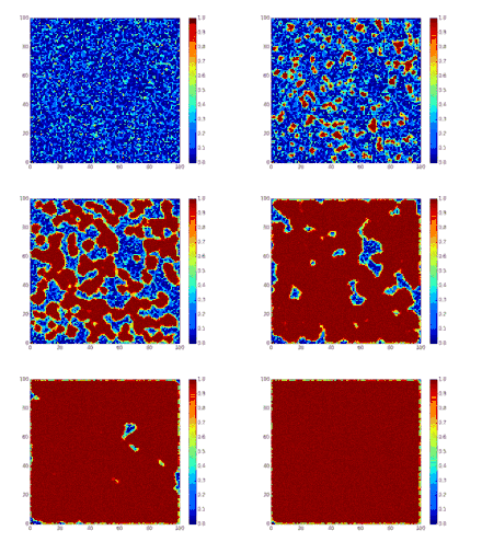
These variables (S, I, and R) represent the number of people in each compartment at a particular time. To represent that the number of susceptible, infectious and removed individuals may vary over time (even if the total population size remains constant), we make the precise numbers a function of t (time): S(t), I(t) and R(t). For a specific disease in a specific population, these functions may be worked out in order to predict possible outbreaks and bring them under control.[11]
As implied by the variable function of t, the model is dynamic in that the numbers in each compartment may fluctuate over time. The importance of this dynamic aspect is most obvious in an endemic disease with a short infectious period, such as measles in the UK prior to the introduction of a vaccine in 1968. Such diseases tend to occur in cycles of outbreaks due to the variation in number of susceptibles (S(t)) over time. During an epidemic, the number of susceptible individuals falls rapidly as more of them are infected and thus enter the infectious and removed compartments. The disease cannot break out again until the number of susceptibles has built back up, e.g. as a result of offspring being born into the susceptible compartment.
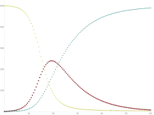
Each member of the population typically progresses from susceptible to infectious to recovered. This can be shown as a flow diagram in which the boxes represent the different compartments and the arrows the transition between compartments, i.e.
Transition rates
For the full specification of the model, the arrows should be labeled with the transition rates between compartments. Between S and I, the transition rate is assumed to be d(S/N)/dt = -βSI/N2, where N is the total population, β is the average number of contacts per person per time, multiplied by the probability of disease transmission in a contact between a susceptible and an infectious subject, and SI/N2 is the fraction of those contacts between an infectious and susceptible individual which result in the susceptible person becoming infected. (This is mathematically similar to the law of mass action in chemistry in which random collisions between molecules result in a chemical reaction and the fractional rate is proportional to the concentration of the two reactants).
Between I and R, the transition rate is assumed to be proportional to the number of infectious individuals which is γI. This is equivalent to assuming that the probability of an infectious individual recovering in any time interval dt is simply γdt. If an individual is infectious for an average time period D, then γ = 1/D. This is also equivalent to the assumption that the length of time spent by an individual in the infectious state is a random variable with an exponential distribution. The "classical" SIR model may be modified by using more complex and realistic distributions for the I-R transition rate (e.g. the Erlang distribution[13]).
For the special case in which there is no removal from the infectious compartment (γ=0), the SIR model reduces to a very simple SI model, which has a logistic solution, in which every individual eventually becomes infected.
The SIR model without birth and death
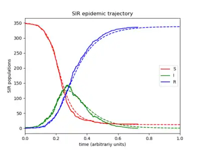
The dynamics of an epidemic, for example, the flu, are often much faster than the dynamics of birth and death, therefore, birth and death are often omitted in simple compartmental models. The SIR system without so-called vital dynamics (birth and death, sometimes called demography) described above can be expressed by the following system of ordinary differential equations:[8][14]

where is the stock of susceptible population, is the stock of infected, is the stock of removed population (either by death or recovery), and is the sum of these three.
This model was for the first time proposed by William Ogilvy Kermack and Anderson Gray McKendrick as a special case of what we now call Kermack–McKendrick theory, and followed work McKendrick had done with Ronald Ross.
This system is non-linear, however it is possible to derive its analytic solution in implicit form.[7] Firstly note that from:
it follows that:
expressing in mathematical terms the constancy of population . Note that the above relationship implies that one need only study the equation for two of the three variables.
Secondly, we note that the dynamics of the infectious class depends on the following ratio:
the so-called basic reproduction number (also called basic reproduction ratio). This ratio is derived as the expected number of new infections (these new infections are sometimes called secondary infections) from a single infection in a population where all subjects are susceptible.[15][16] This idea can probably be more readily seen if we say that the typical time between contacts is , and the typical time until removal is . From here it follows that, on average, the number of contacts by an infectious individual with others before the infectious has been removed is:
There is also an effective reproduction number , which is similarly defined but in a population made up of both susceptible and infected individuals. The basic reproduction rate quantifies the initial contagiousness of the disease, but the effective reproduction number is a time-dependent rate. [17]
By dividing the first differential equation by the third, separating the variables and integrating we get
where and are the initial numbers of, respectively, susceptible and removed subjects. Writing for the initial proportion of susceptible individuals, and and for the proportion of susceptible and removed individuals respectively in the limit one has
(note that the infectious compartment empties in this limit). This transcendental equation has a solution in terms of the Lambert W function,[18] namely
This shows that at the end of an epidemic that conforms to the simple assumptions of the SIR model, unless , not all individuals of the population have been removed, so some must remain susceptible. A driving force leading to the end of an epidemic is a decline in the number of infectious individuals. The epidemic does not typically end because of a complete lack of susceptible individuals.
The role of both the basic reproduction number and the initial susceptibility are extremely important. In fact, upon rewriting the equation for infectious individuals as follows:
it yields that if:
then:
i.e., there will be a proper epidemic outbreak with an increase of the number of the infectious (which can reach a considerable fraction of the population). On the contrary, if
then
i.e., independently from the initial size of the susceptible population the disease can never cause a proper epidemic outbreak. As a consequence, it is clear that both the basic reproduction number and the initial susceptibility are extremely important.
The force of infection
Note that in the above model the function:
models the transition rate from the compartment of susceptible individuals to the compartment of infectious individuals, so that it is called the force of infection. However, for large classes of communicable diseases it is more realistic to consider a force of infection that does not depend on the absolute number of infectious subjects, but on their fraction (with respect to the total constant population ):
Capasso[19] and, afterwards, other authors have proposed nonlinear forces of infection to model more realistically the contagion process.
Exact analytical solutions to the SIR model
In 2014, Harko and coauthors derived an exact so-called analytical solution (involving an integral that can only be calculated numerically) to the SIR model.[7] In the case without vital dynamics setup, for , etc., it corresponds to the following time parametrization
for
with initial conditions
where satisfies . By the transcendental equation for above, it follows that , if and .
An equivalent so-called analytical solution (involving an integral that can only be calculated numerically) found by Miller[20][21] yields
Here can be interpreted as the expected number of transmissions an individual has received by time . The two solutions are related by .
Effectively the same result can be found in the original work by Kermack and McKendrick.[4]
These solutions may be easily understood by noting that all of the terms on the right-hand sides of the original differential equations are proportional to . The equations may thus be divided through by , and the time rescaled so that the differential operator on the left-hand side becomes simply , where , i.e. . The differential equations are now all linear, and the third equation, of the form const., shows that and (and above) are simply linearly related.
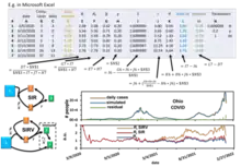
A highly accurate analytic approximant of the SIR model as well as exact analytic expressions for the final values , , and were provided by Kröger and Schlickeiser,[9] so that there is no need to perform a numerical integration to solve the SIR model (a simplified example practice on COVID-19 numerical simulation using Microsoft Excel can be found here [22]), to obtain its parameters from existing data, or to predict the future dynamics of an epidemics modeled by the SIR model. The approximant involves the Lambert W function which is part of all basic data visualization software such as Microsoft Excel, MATLAB, and Mathematica.
While Kendall[5] considered the so-called all-time SIR model where the initial conditions , , and are coupled through the above relations, Kermack and McKendrick[4] proposed to study the more general semi-time case, for which and are both arbitrary. This latter version, denoted as semi-time SIR model,[9] makes predictions only for future times . An analytic approximant and exact expressions for the final values are available for the semi-time SIR model as well.[10]
Numerical solutions to the SIR model with approximations
Numerical solutions to the SIR model can be found in the literature. An example is using the model to analyze COVID-19 spreading data. [22] [23] Three reproduction numbers can be pulled out from the data analyzed with numerical approximation,
- the real-time reproduction number:
- and the real-time effective reproduction number:
represents the speed of reproduction rate at the beginning of the spreading when all populations are assumed susceptible, e.g. if and meaning one infectious person on average infects 0.4 susceptible people per day and recovers in 1/0.2=5 days. Thus when this person recovered, there are two people still infectious directly got from this person and , i.e. the number of infectious people doubled in one cycle of 5 days. The data simulated by the model with or real data fitted will yield a doubling of the number of infectious people faster than 5 days because the two infected people are infecting people. From the SIR model, we can tell that is determined by the nature of the disease and also a function of the interactive frequency between the infectious person with the susceptible people and also the intensity/duration of the interaction like how close they interact for how long and whether or not they both wear masks, thus, it changes over time when the average behavior of the carriers and susceptible people changes. The model use to represent these factors but it indeed is referenced to the initial stage when no action is taken to prevent the spread and all population is susceptible, thus all changes are absorbed by the change of .
is usually more stable over time assuming when the infectious person shows symptoms, she/he will seek medical attention or be self-isolated. So if we find changes, most probably the behaviors of people in the community have changed from their normal patterns before the outbreak, or the disease has mutated to a new form. Costive massive detection and isolation of susceptible close contacts have effects on reducing but whose efficiencies are under debate. This debate is largely on the uncertainty of the number of days reduced from after infectious or detectable whichever comes first to before a symptom shows up for an infected susceptible person. If the person is infectious after symptoms show up, or detection only works for a person with symptoms, then these prevention methods are not necessary, and self-isolation and/or medical attention is the best way to cut the values. The typical onset of the COVID-19 infectious period is in the order of one day from the symptoms showing up, making massive detection with typical frequency in a few days useless.
does not tell us whether or not the spreading will speed up or slow down in the latter stages when the fraction of susceptible people in the community has dropped significantly after recovery or vaccination. corrects this dilution effect by multiplying the fraction of the susceptible population over the total population. It corrects the effective/transmissible interaction between an infectious person and the rest of the community when many of the interaction is immune in the middle to late stages of the disease spreading. Thus, when , we will see an exponential-like outbreak; when , a steady state reached and no number of infectious people changes over time; and when , the disease decays and fades away over time.
Using the differential equations of the SIR model and converting them to numerical discrete forms, one can set up the recursive equations and calculate the S, I, and R populations with any given initial conditions but accumulate errors over a long calculation time from the reference point. Sometimes a convergence test is needed to estimate the errors. Given a set of initial conditions and the disease-spreading data, one can also fit the data with the SIR model and pull out the three reproduction numbers when the errors are usually negligible due to the short time step from the reference point.[22][23] Any point of the time can be used as the initial condition to predict the future after it using this numerical model with assumption of time-evolved parameters such as population, , and . However, away from this reference point, errors will accumulate over time thus convergence test is needed to find an optimal time step for more accurate results.
Among these three reproduction numbers, is very useful to judge the control pressure, e.g., a large value meaning the disease will spread very fast and is very difficult to control. is most useful in predicting future trends, for example, if we know the social interactions have reduced 50% frequently from that before the outbreak and the interaction intensities among people are the same, then we can set . If social distancing and masks add another 50% cut in infection efficiency, we can set . will perfectly correlate with the waves of the spreading and whenever , the spreading accelerates, and when , the spreading slows down thus useful to set a prediction on the short term trends. Also, it can be used to directly calculate the threshold population of vaccination/immunization for the herd immunity stage by setting .
The SIR model with vital dynamics and constant population
Consider a population characterized by a death rate and birth rate , and where a communicable disease is spreading.[8] The model with mass-action transmission is:
for which the disease-free equilibrium (DFE) is:
In this case, we can derive a basic reproduction number:
which has threshold properties. In fact, independently from biologically meaningful initial values, one can show that:
The point EE is called the Endemic Equilibrium (the disease is not totally eradicated and remains in the population). With heuristic arguments, one may show that may be read as the average number of infections caused by a single infectious subject in a wholly susceptible population, the above relationship biologically means that if this number is less than or equal to one the disease goes extinct, whereas if this number is greater than one the disease will remain permanently endemic in the population.
The SIR model
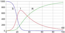
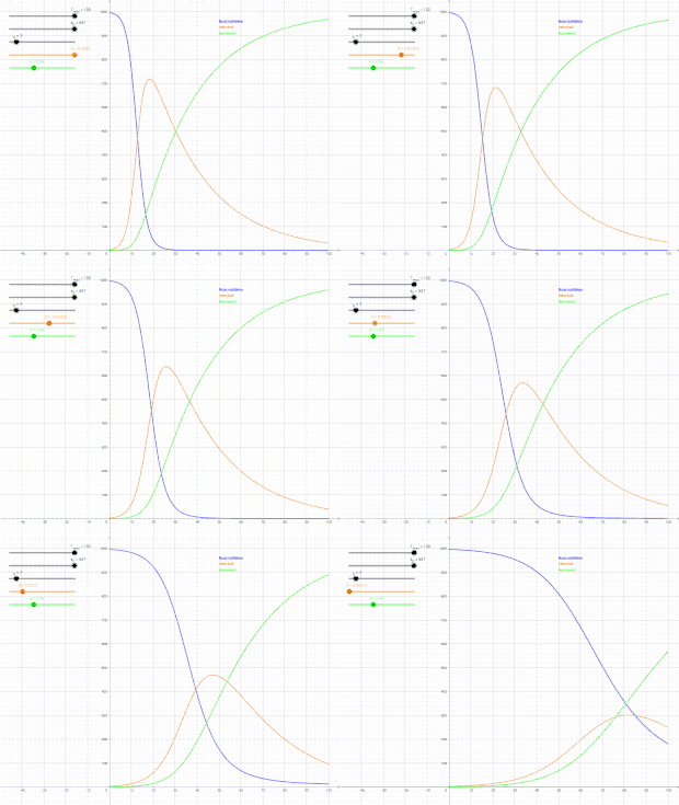
In 1927, W. O. Kermack and A. G. McKendrick created a model in which they considered a fixed population with only three compartments: susceptible, ; infected, ; and recovered, . The compartments used for this model consist of three classes:[4]
- is used to represent the individuals not yet infected with the disease at time t, or those susceptible to the disease of the population.
- denotes the individuals of the population who have been infected with the disease and are capable of spreading the disease to those in the susceptible category.
- is the compartment used for the individuals of the population who have been infected and then removed from the disease, either due to immunization or due to death. Those in this category are not able to be infected again or to transmit the infection to others.
The flow of this model may be considered as follows:
Using a fixed population, in the three functions resolves that the value should remain constant within the simulation, if a simulation is used to solve the SIR model. Alternatively, the analytic approximant[9] can be used without performing a simulation. The model is started with values of , and . These are the number of people in the susceptible, infected and removed categories at time equals zero. If the SIR model is assumed to hold at all times, these initial conditions are not independent.[9] Subsequently, the flow model updates the three variables for every time point with set values for and . The simulation first updates the infected from the susceptible and then the removed category is updated from the infected category for the next time point (t=1). This describes the flow persons between the three categories. During an epidemic the susceptible category is not shifted with this model, changes over the course of the epidemic and so does . These variables determine the length of the epidemic and would have to be updated with each cycle.
Several assumptions were made in the formulation of these equations: First, an individual in the population must be considered as having an equal probability as every other individual of contracting the disease with a rate of and an equal fraction of people that an individual makes contact with per unit time. Then, let be the multiplication of and . This is the transmission probability times the contact rate. Besides, an infected individual makes contact with persons per unit time whereas only a fraction, of them are susceptible. Thus, we have every infective can infect susceptible persons, and therefore, the whole number of susceptibles infected by infectives per unit time is . For the second and third equations, consider the population leaving the susceptible class as equal to the number entering the infected class. However, a number equal to the fraction (which represents the mean recovery/death rate, or the mean infective period) of infectives are leaving this class per unit time to enter the removed class. These processes which occur simultaneously are referred to as the Law of Mass Action, a widely accepted idea that the rate of contact between two groups in a population is proportional to the size of each of the groups concerned. Finally, it is assumed that the rate of infection and recovery is much faster than the time scale of births and deaths and therefore, these factors are ignored in this model.[24]
Steady-state solutions
The expected duration of susceptibility will be where reflects the time alive (life expectancy) and reflects the time in the susceptible state before becoming infected, which can be simplified[25] to:
such that the number of susceptible persons is the number entering the susceptible compartment times the duration of susceptibility:
Analogously, the steady-state number of infected persons is the number entering the infected state from the susceptible state (number susceptible, times rate of infection) times the duration of infectiousness :
Other compartmental models
There are many modifications of the SIR model, including those that include births and deaths, where upon recovery there is no immunity (SIS model), where immunity lasts only for a short period of time (SIRS), where there is a latent period of the disease where the person is not infectious (SEIS and SEIR), and where infants can be born with immunity (MSIR). Compartmental models can also be used to model multiple risk groups, and even the interaction of multiple pathogens.[26]
Variations on the basic SIR model
The SIS model
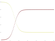
Some infections, for example, those from the common cold and influenza, do not confer any long-lasting immunity. Such infections may give temporary resistance but do not give long-term immunity upon recovery from infection, and individuals become susceptible again.

We have the model:
Note that denoting with N the total population it holds that:
- .
It follows that:
- ,
i.e. the dynamics of infectious is ruled by a logistic function, so that :
It is possible to find an analytical solution to this model (by making a transformation of variables: and substituting this into the mean-field equations),[27] such that the basic reproduction rate is greater than unity. The solution is given as
- .
where is the endemic infectious population, , and . As the system is assumed to be closed, the susceptible population is then .
Whenever the integer nature of the number of agents is evident (populations with fewer than tens of thousands of individuals), inherent fluctuations in the disease spreading process caused by discrete agents result in uncertainties.[28] In this scenario, the evolution of the disease predicted by compartmental equations deviates significantly from the observed results. These uncertainties may even cause the epidemic to end earlier than predicted by the compartmental equations.
As a special case, one obtains the usual logistic function by assuming . This can be also considered in the SIR model with , i.e. no removal will take place. That is the SI model.[29] The differential equation system using thus reduces to:
In the long run, in the SI model, all individuals will become infected.
The SIRD model
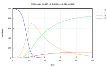
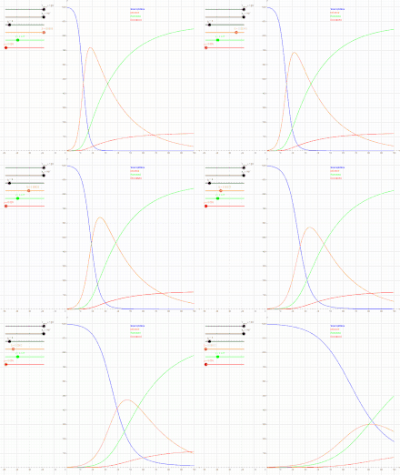
The Susceptible-Infectious-Recovered-Deceased model differentiates between Recovered (meaning specifically individuals having survived the disease and now immune) and Deceased.[15] The SIRD model has semi analytical solutions based on the four parts method.[30] This model uses the following system of differential equations:
where are the rates of infection, recovery, and mortality, respectively.[31]
The SIRV model
The Susceptible-Infectious-Recovered-Vaccinated model is an extended SIR model that accounts for vaccination of the susceptible population.[32] This model uses the following system of differential equations:

where are the rates of infection, recovery, and vaccination, respectively. For the semi-time initial conditions , , and constant ratios and the model had been solved approximately.[32] The occurrence of a pandemic outburst requires and there is a critical reduced vaccination rate beyond which the steady-state size of the susceptible compartment remains relatively close to . Arbitrary initial conditions satisfying can be mapped to the solved special case with .[32]
The numerical solution of this model to calculate the real-time reproduction number of COVID-19 can be practiced based on information from the different populations in a community.[23] Numerical solution is a commonly used method to analyze complicated kinetic networks when the analytical solution is difficult to obtain or limited by requirements such as boundary conditions or special parameters. It uses recursive equations to calculate the next step by converting the numerical integration into Riemann sum of discrete time steps e.g., use yesterday's principal and interest rate to calculate today's interest which assumes the interest rate is fixed during the day. The calculation contains projected errors if the analytical corrections on the numerical step size are not included, e.g. when the interest rate of annual collection is simplified to 12 times the monthly rate, a projected error is introduced. Thus the calculated results will carry accumulative errors when the time step is far away from the reference point and a convergence test is needed to estimate the error. However, this error is usually acceptable for data fitting. When fitting a set of data with a close time step, the error is relatively small because the reference point is nearby compared to when predicting a long period of time after a reference point. Once the real-time is pulled out, one can compare it to the basic reproduction number . Before the vaccination, gives the policy maker and general public a measure of the efficiency of social mitigation activities such as social distancing and face masking simply by dividing . Under massive vaccination, the goal of disease control is to reduce the effective reproduction number , where is the number of susceptible population at the time and is the total population. When , the spreading decays and daily infected cases go down.
The MSIR model
For many infections, including measles, babies are not born into the susceptible compartment but are immune to the disease for the first few months of life due to protection from maternal antibodies (passed across the placenta and additionally through colostrum). This is called passive immunity. This added detail can be shown by including an M class (for maternally derived immunity) at the beginning of the model.

To indicate this mathematically, an additional compartment is added, M(t). This results in the following differential equations:
Carrier state
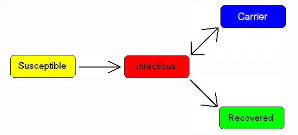
Some people who have had an infectious disease such as tuberculosis never completely recover and continue to carry the infection, whilst not suffering the disease themselves. They may then move back into the infectious compartment and suffer symptoms (as in tuberculosis) or they may continue to infect others in their carrier state, while not suffering symptoms. The most famous example of this is probably Mary Mallon, who infected 22 people with typhoid fever. The carrier compartment is labelled C.
The SEIR model
For many important infections, there is a significant latency period during which individuals have been infected but are not yet infectious themselves. During this period the individual is in compartment E (for exposed).

Assuming that the latency period is a random variable with exponential distribution with parameter (i.e. the average latency period is ), and also assuming the presence of vital dynamics with birth rate equal to death rate (so that the total number is constant), we have the model:
We have but this is only constant because of the simplifying assumption that birth and death rates are equal; in general is a variable.
For this model, the basic reproduction number is:
Similarly to the SIR model, also, in this case, we have a Disease-Free-Equilibrium (N,0,0,0) and an Endemic Equilibrium EE, and one can show that, independently from biologically meaningful initial conditions
it holds that:
In case of periodically varying contact rate the condition for the global attractiveness of DFE is that the following linear system with periodic coefficients:
is stable (i.e. it has its Floquet's eigenvalues inside the unit circle in the complex plane).
The SEIS model
The SEIS model is like the SEIR model (above) except that no immunity is acquired at the end.
In this model an infection does not leave any immunity thus individuals that have recovered return to being susceptible, moving back into the S(t) compartment. The following differential equations describe this model:
The MSEIR model
For the case of a disease, with the factors of passive immunity, and a latency period there is the MSEIR model.
The MSEIRS model
An MSEIRS model is similar to the MSEIR, but the immunity in the R class would be temporary, so that individuals would regain their susceptibility when the temporary immunity ended.
Variable contact rates
It is well known that the probability of getting a disease is not constant in time. As a pandemic progresses, reactions to the pandemic may change the contact rates which are assumed constant in the simpler models. Counter-measures such as masks, social distancing and lockdown will alter the contact rate in a way to reduce the speed of the pandemic.
In addition, Some diseases are seasonal, such as the common cold viruses, which are more prevalent during winter. With childhood diseases, such as measles, mumps, and rubella, there is a strong correlation with the school calendar, so that during the school holidays the probability of getting such a disease dramatically decreases. As a consequence, for many classes of diseases, one should consider a force of infection with periodically ('seasonal') varying contact rate
with period T equal to one year.
Thus, our model becomes
(the dynamics of recovered easily follows from ), i.e. a nonlinear set of differential equations with periodically varying parameters. It is well known that this class of dynamical systems may undergo very interesting and complex phenomena of nonlinear parametric resonance. It is easy to see that if:
whereas if the integral is greater than one the disease will not die out and there may be such resonances. For example, considering the periodically varying contact rate as the 'input' of the system one has that the output is a periodic function whose period is a multiple of the period of the input. This allowed to give a contribution to explain the poly-annual (typically biennial) epidemic outbreaks of some infectious diseases as interplay between the period of the contact rate oscillations and the pseudo-period of the damped oscillations near the endemic equilibrium. Remarkably, in some cases, the behavior may also be quasi-periodic or even chaotic.
SIR model with diffusion
Spatiotemporal compartmental models describe not the total number, but the density of susceptible/infective/recovered persons. Consequently, they also allow to model the distribution of infected persons in space. In most cases, this is done by combining the SIR model with a diffusion equation
where , and are diffusion constants. Thereby, one obtains a reaction-diffusion equation. (Note that, for dimensional reasons, the parameter has to be changed compared to the simple SIR model.) Early models of this type have been used to model the spread of the black death in Europe.[34] Extensions of this model have been used to incorporate, e.g., effects of nonpharmaceutical interventions such as social distancing.[35]
Interacting Subpopulation SEIR Model
As social contacts, disease severity and lethality, as well as the efficacy of prophylactic measures may differ substantially between interacting subpopulations, e.g., the elderly versus the young, separate SEIR models for each subgroup may be used that are mutually connected through interaction links.[33] Such Interacting Subpopulation SEIR models have been used for modeling the COVID-19 pandemic at continent scale to develop personalized, accelerated, subpopulation-targeted vaccination strategies[36] that promise a shortening of the pandemic and a reduction of case and death counts in the setting of limited access to vaccines during a wave of virus Variants of Concern.
SIR Model on Networks
The SIR model has been studied on networks of various kinds in order to model a more realistic form of connection than the homogeneous mixing condition which is usually required. A simple model for epidemics on networks in which an individual has a probability p of being infected by each of his infected neighbors in a given time step leads to results similar to giant component formation on Erdos Renyi random graphs.[37]
SIRSS model - combination of SIR with modelling of social stress
Dynamics of epidemics depend on how people's behavior changes in time. For example, at the beginning of the epidemic, people are ignorant and careless, then, after the outbreak of epidemics and alarm, they begin to comply with the various restrictions and the spreading of epidemics may decline. Over time, some people get tired/frustrated by the restrictions and stop following them (exhaustion), especially if the number of new cases drops down. After resting for some time, they can follow the restrictions again. But during this pause the second wave can come and become even stronger than the first one. Social dynamics should be considered. The social physics models of social stress complement the classical epidemics models.[38]
The simplest SIR-social stress (SIRSS) model is organised as follows. The susceptible individuals (S) can be split in three subgroups by the types of behavior: ignorant or unaware of the epidemic (Sign), rationally resistant (Sres), and exhausted (Sexh) that do not react on the external stimuli (this is a sort of refractory period). In other words: S(t) = Sign(t) + Sres(t) + Sexh(t). Symbolically, the social stress model can be presented by the "reaction scheme" (where I denotes the infected individuals):
- – mobilization reaction (the autocatalytic form here means that the transition rate is proportional to the square of the infected fraction I);
- – exhaustion process due to fatigue from anti-epidemic restrictions;
- – slow relaxation to the initial state (end of the refractory period).
The main SIR epidemic reaction
has different reaction rate constants for Sign, Sres, and Sexh. Presumably, for Sres, is lower than for Sign and Sign.
The differences between countries are concentrated in two kinetic constants: the rate of mobilization and the rate of exhaustion calculated for COVID-19 epidemic in 13 countries.[38] These constants for this epidemic in all countries can be extracted by the fitting of the SIRSS model to publicly available data [39]
The KdV-SIR equation
Based on the classical SIR model, a Korteweg-de Vries (KdV)–SIR equation and its analytical solution have been proposed to illustrate the fundamental dynamics of an epidemic wave, the dependence of solutions on parameters, and the dependence of predictability horizons on various types of solutions.[40] The KdV-SIR equation is written as follows:
.
Here,
,
,
and
.
indicates the initial value of the state variable . Parameters (σ-naught) and (R-naught) are the time-independent relative growth rate and basic reproduction number, respectively. presents the maximum of the state variables (for the number of infected persons). An analytical solution to the KdV-SIR equation is written as follows:
,
which represents a solitary wave solution.
Modelling vaccination
The SIR model can be modified to model vaccination.[41] Typically these introduce an additional compartment to the SIR model, , for vaccinated individuals. Below are some examples.
Vaccinating newborns
In presence of a communicable diseases, one of the main tasks is that of eradicating it via prevention measures and, if possible, via the establishment of a mass vaccination program. Consider a disease for which the newborn are vaccinated (with a vaccine giving lifelong immunity) at a rate :
where is the class of vaccinated subjects. It is immediate to show that:
thus we shall deal with the long term behavior of and , for which it holds that:
In other words, if
the vaccination program is not successful in eradicating the disease, on the contrary, it will remain endemic, although at lower levels than the case of absence of vaccinations. This means that the mathematical model suggests that for a disease whose basic reproduction number may be as high as 18 one should vaccinate at least 94.4% of newborns in order to eradicate the disease.
Vaccination and information
Modern societies are facing the challenge of "rational" exemption, i.e. the family's decision to not vaccinate children as a consequence of a "rational" comparison between the perceived risk from infection and that from getting damages from the vaccine. In order to assess whether this behavior is really rational, i.e. if it can equally lead to the eradication of the disease, one may simply assume that the vaccination rate is an increasing function of the number of infectious subjects:
In such a case the eradication condition becomes:
i.e. the baseline vaccination rate should be greater than the "mandatory vaccination" threshold, which, in case of exemption, cannot hold. Thus, "rational" exemption might be myopic since it is based only on the current low incidence due to high vaccine coverage, instead taking into account future resurgence of infection due to coverage decline.
Vaccination of non-newborns
In case there also are vaccinations of non newborns at a rate ρ the equation for the susceptible and vaccinated subject has to be modified as follows:
leading to the following eradication condition:
Pulse vaccination strategy
This strategy repeatedly vaccinates a defined age-cohort (such as young children or the elderly) in a susceptible population over time. Using this strategy, the block of susceptible individuals is then immediately removed, making it possible to eliminate an infectious disease, (such as measles), from the entire population. Every T time units a constant fraction p of susceptible subjects is vaccinated in a relatively short (with respect to the dynamics of the disease) time. This leads to the following impulsive differential equations for the susceptible and vaccinated subjects:
It is easy to see that by setting I = 0 one obtains that the dynamics of the susceptible subjects is given by:
and that the eradication condition is:
The influence of age: age-structured models
Age has a deep influence on the disease spread rate in a population, especially the contact rate. This rate summarizes the effectiveness of contacts between susceptible and infectious subjects. Taking into account the ages of the epidemic classes (to limit ourselves to the susceptible-infectious-removed scheme) such that:
(where is the maximum admissible age) and their dynamics is not described, as one might think, by "simple" partial differential equations, but by integro-differential equations:
where:
is the force of infection, which, of course, will depend, though the contact kernel on the interactions between the ages.
Complexity is added by the initial conditions for newborns (i.e. for a=0), that are straightforward for infectious and removed:
but that are nonlocal for the density of susceptible newborns:
where are the fertilities of the adults.
Moreover, defining now the density of the total population one obtains:
In the simplest case of equal fertilities in the three epidemic classes, we have that in order to have demographic equilibrium the following necessary and sufficient condition linking the fertility with the mortality must hold:
and the demographic equilibrium is
automatically ensuring the existence of the disease-free solution:
A basic reproduction number can be calculated as the spectral radius of an appropriate functional operator.
Other considerations within compartmental epidemic models
Vertical transmission
In the case of some diseases such as AIDS and hepatitis B, it is possible for the offspring of infected parents to be born infected. This transmission of the disease down from the mother is referred to as vertical transmission. The influx of additional members into the infected category can be considered within the model by including a fraction of the newborn members in the infected compartment.[42]
Vector transmission
Diseases transmitted from human to human indirectly, i.e. malaria spread by way of mosquitoes, are transmitted through a vector. In these cases, the infection transfers from human to insect and an epidemic model must include both species, generally requiring many more compartments than a model for direct transmission.[42][43]
Others
Other occurrences which may need to be considered when modeling an epidemic include things such as the following:[42]
- Non-homogeneous mixing
- Variable infectivity
- Distributions that are spatially non-uniform
- Diseases caused by macroparasites
Deterministic versus stochastic epidemic models
It is important to stress that the deterministic models presented here are valid only in case of sufficiently large populations, and as such should be used cautiously.[44] [45]
To be more precise, these models are only valid in the thermodynamic limit, where the population is effectively infinite. In stochastic models, the long-time endemic equilibrium derived above, does not hold, as there is a finite probability that the number of infected individuals drops below one in a system. In a true system then, the pathogen may not propagate, as no host will be infected. But, in deterministic mean-field models, the number of infected can take on real, namely, non-integer values of infected hosts, and the number of hosts in the model can be less than one, but more than zero, thereby allowing the pathogen in the model to propagate. The reliability of compartmental models is limited to compartmental applications.
One of the possible extensions of mean-field models considers the spreading of epidemics on a network based on percolation theory concepts.[37] Stochastic epidemic models have been studied on different networks[46][47][48] and more recently applied to the COVID-19 pandemic.[49]
See also
References
- Ross R (1 February 1916). "An application of the theory of probabilities to the study of a priori pathometry.—Part I". Proceedings of the Royal Society of London. Series A, Containing Papers of a Mathematical and Physical Character. 92 (638): 204–230. Bibcode:1916RSPSA..92..204R. doi:10.1098/rspa.1916.0007.
- Ross R, Hudson H (3 May 1917). "An application of the theory of probabilities to the study of a priori pathometry.—Part II". Proceedings of the Royal Society of London. Series A, Containing Papers of a Mathematical and Physical Character. 93 (650): 212–225. Bibcode:1917RSPSA..93..212R. doi:10.1098/rspa.1917.0014.
- Ross R, Hudson H (1917). "An application of the theory of probabilities to the study of a priori pathometry.—Part III". Proceedings of the Royal Society of London. Series A, Containing Papers of a Mathematical and Physical Character. 89 (621): 225–240. Bibcode:1917RSPSA..93..225R. doi:10.1098/rspa.1917.0015.
- Kermack WO, McKendrick AG (1927). "A Contribution to the Mathematical Theory of Epidemics". Proceedings of the Royal Society of London. Series A, Containing Papers of a Mathematical and Physical Character. 115 (772): 700–721. Bibcode:1927RSPSA.115..700K. doi:10.1098/rspa.1927.0118.
- Kendall DG (1956). "Deterministic and stochastic epidemics in closed populations". Proceedings of the Third Berkeley Symposium on Mathematical Statistics and Probability: Contributions to Biology and Problems of Health. 4: 149–165. doi:10.1525/9780520350717-011. ISBN 9780520350717. MR 0084936. Zbl 0070.15101.
- Engelmann, Lukas (2021-08-30). "A box, a trough and marbles: How the Reed-Frost epidemic theory shaped epidemiological reasoning in the 20th century". History and Philosophy of the Life Sciences. 43 (3): 105. doi:10.1007/s40656-021-00445-z. ISSN 1742-6316. PMC 8404547. PMID 34462807.
- Harko T, Lobo FS, Mak MK (2014). "Exact analytical solutions of the Susceptible-Infected-Recovered (SIR) epidemic model and of the SIR model with equal death and birth rates". Applied Mathematics and Computation. 236: 184–194. arXiv:1403.2160. Bibcode:2014arXiv1403.2160H. doi:10.1016/j.amc.2014.03.030. S2CID 14509477.
- Beckley R, Weatherspoon C, Alexander M, Chandler M, Johnson A, Bhatt GS (2013). "Modeling epidemics with differential equations" (PDF). Tennessee State University Internal Report. Retrieved July 19, 2020.
- Kröger M, Schlickeiser R (2020). "Analytical solution of the SIR-model for the temporal evolution of epidemics. Part A: Time-independent reproduction factor". Journal of Physics A. 53 (50): 505601. Bibcode:2020JPhA...53X5601K. doi:10.1088/1751-8121/abc65d. S2CID 225555567.
- Schlickeiser R, Kröger M (2021). "Analytical solution of the SIR-model for the temporal evolution of epidemics. Part B: Semi-time case". Journal of Physics A. 54 (17): 175601. Bibcode:2021JPhA...54q5601S. doi:10.1088/1751-8121/abed66.
- Yang W, Zhang D, Peng L, Zhuge C, Hong L (2020). "Rational evaluation of various epidemic models based on the COVID-19 data of China". arXiv:2003.05666v1 [q-bio.PE].
- Shirzad K.; Viney C. (2023). "A critical review on applications of the Avrami equation beyond materials science". Journal of the Royal Society Interface. 20 (203). doi:10.1098/rsif.2023.0242. PMC 10282574. PMID 37340781.
- Krylova O, Earn DJ (July 2013). "Effects of the infectious period distribution on predicted transitions in childhood disease dynamics". Journal of the Royal Society, Interface. 10 (84): 20130098. doi:10.1098/rsif.2013.0098. PMC 3673147. PMID 23676892.
- Hethcote H (2000). "The Mathematics of Infectious Diseases". SIAM Review. 42 (4): 599–653. Bibcode:2000SIAMR..42..599H. doi:10.1137/s0036144500371907. S2CID 10836889.
- Bailey, Norman T. J. (1975). The mathematical theory of infectious diseases and its applications (2nd ed.). London: Griffin. ISBN 0-85264-231-8.
- Sonia Altizer; Nunn, Charles (2006). Infectious diseases in primates: behavior, ecology and evolution. Oxford Series in Ecology and Evolution. Oxford [Oxfordshire]: Oxford University Press. ISBN 0-19-856585-2.
- Shirzad K.; Viney C. (2023). "A critical review on applications of the Avrami equation beyond materials science". Journal of the Royal Society Interface. 20 (203). doi:10.1098/rsif.2023.0242. PMC 10282574. PMID 37340781.
- Wolfram Research, Inc. "Mathematica, Version 12.1". Champaign IL, 2020.
- Capasso V (1993). Mathematical Structure of Epidemic Systems. Berlin: Springer. ISBN 3-540-56526-4.
- Miller JC (September 2012). "A note on the derivation of epidemic final sizes". Bulletin of Mathematical Biology. 74 (9): 2125–2141. doi:10.1007/s11538-012-9749-6. PMC 3506030. PMID 22829179.
Section 4.1
- Miller JC (February 2017). "Mathematical models of SIR disease spread with combined non-sexual and sexual transmission routes". Infectious Disease Modelling. 2 (1): 35–55. doi:10.1016/j.idm.2016.12.003. PMC 5963332. PMID 29928728.
Section 2.1.3
- Hart KD, Thompson C, Burger C, Hardwick D, Michaud AH, Bulushi A, Pridemore C, Ward C, Chen J (2021). "Remote Learning of COVID-19 Kinetic Analysis in a Physical Chemistry Laboratory Class". ACS Omega. 6 (43): 29223–29232. doi:10.1021/acsomega.1c04842. PMC 8547164. PMID 34723043.
- Smith DK, Lauro K, Kelly D, Fish J, Lintelman E, McEwen D, Smith C, Stecz M, Ambagaspitiya TD, Chen J (2022). "Teaching Undergraduate Physical Chemistry Lab with Kinetic Analysis of COVID-19 in the United States". Journal of Chemical Education. 99 (10): 3471–3477. Bibcode:2022JChEd..99.3471S. doi:10.1021/acs.jchemed.2c00416. PMC 9799982. PMID 36589277. S2CID 251484056.
- Padua RN, Tulang AB (2 December 2010). "A Density–Dependent Epidemiological Model for the Spread of Infectious Diseases". Liceo Journal of Higher Education Research. 6 (2). doi:10.7828/ljher.v6i2.62.
- May RM, Anderson B (1992-09-24). Infectious Diseases of Humans: Dynamics and Control (Revised ed.). Oxford: Oxford University Press. ISBN 9780198540403.
- von Csefalvay, Chris (2023-01-01), von Csefalvay, Chris (ed.), "3 - Host factors: Who gets sick and why", Computational Modeling of Infectious Disease, Academic Press, pp. 93–119, doi:10.1016/b978-0-32-395389-4.00012-8, ISBN 978-0-323-95389-4, retrieved 2023-03-02
- Hethcote HW (1989). "Three Basic Epidemiological Models". In Levin SA, Hallam TG, Gross LJ (eds.). Applied Mathematical Ecology. Biomathematics. Vol. 18. Berlin: Springer. pp. 119–144. doi:10.1007/978-3-642-61317-3_5. ISBN 3-540-19465-7.
- Nakamura, G.M.; Cardoso, G.C.; Martinez, A.S. (2020). "Improved susceptible–infectious–susceptible epidemic equations based on uncertainties and autocorrelation functions". Royal Society Open Science. 7 (2): 191504. Bibcode:2020RSOS....791504N. doi:10.1098/rsos.191504. PMC 7062106. PMID 32257317.
- "(p. 19) The SI Model" (PDF).
- Al-Raeei, Marwan (2021). "The basic reproduction number of the new coronavirus pandemic with mortality for India, the Syrian Arab Republic, the United States, Yemen, China, France, Nigeria and Russia with different rate of cases". Clinical Epidemiology and Global Health. 9: 147–149. doi:10.1016/j.cegh.2020.08.005. ISSN 2452-0918. PMC 7438206. PMID 32844133.
- The first and second differential equations are transformed and brought to the same form as for the SIR model above.
- Schlickeiser R, Kröger M (2021). "Analytical Modeling of the Temporal Evolution of Epidemics Outbreaks Accounting for Vaccinations". Physics. 3 (2): 386. Bibcode:2021Physi...3..386S. doi:10.3390/physics3020028. S2CID 233589998.
- Hunziker P (2021-07-24). "Personalized-dose Covid-19 vaccination in a wave of virus Variants of Concern: Trading individual efficacy for societal benefit". Precision Nanomedicine. 4 (3): 805–820. doi:10.33218/001c.26101.
- Noble JV (August 1974). "Geographic and temporal development of plagues". Nature. 250 (5469): 726–729. Bibcode:1974Natur.250..726N. doi:10.1038/250726a0. PMID 4606583. S2CID 4210869.
- Te Vrugt M, Bickmann J, Wittkowski R (November 2020). "Effects of social distancing and isolation on epidemic spreading modeled via dynamical density functional theory". Nature Communications. 11 (1): 5576. arXiv:2003.13967. Bibcode:2020NatCo..11.5576T. doi:10.1038/s41467-020-19024-0. PMC 7643184. PMID 33149128.
- Hunziker P (2021-03-07). "Vaccination strategies for minimizing loss of life in Covid-19 in a Europe lacking vaccines". medRxiv 10.1101/2021.01.29.21250747.
- Croccolo F, Roman HE (October 2020). "Spreading of infections on random graphs: A percolation-type model for COVID-19". Chaos, Solitons and Fractals. 139: 110077. arXiv:2006.10490. Bibcode:2020CSF...13910077C. doi:10.1016/j.chaos.2020.110077. PMC 7332959. PMID 32834619. S2CID 219792089.
- Kastalskiy, IA; Pankratova, EV; Mirkes, EM; et al. (2021). "Social stress drives the multi-wave dynamics of COVID-19 outbreaks". Scientific Reports. 11 (1): 22497. arXiv:2106.08966. Bibcode:2021NatSR..1122497K. doi:10.1038/s41598-021-01317-z. PMC 8602246. PMID 34795311.
- The COVID-19 Data Repository. The Center for Systems Science and Engineering (CSSE) at Johns Hopkins University (JHU); the preprocessed data are here: World in Data project.
- Paxson, Wei; Shen, Bo-Wen (2022-10-01). "A KdV–SIR Equation and Its Analytical Solutions for Solitary Epidemic Waves". International Journal of Bifurcation and Chaos. 32 (13): 2250199–2250780. Bibcode:2022IJBC...3250199P. doi:10.1142/S0218127422501991. ISSN 0218-1274. S2CID 253314121.
- Gao S, Teng Z, Nieto JJ, Torres A (2007). "Analysis of an SIR epidemic model with pulse vaccination and distributed time delay". Journal of Biomedicine & Biotechnology. 2007: 64870. doi:10.1155/2007/64870. PMC 2217597. PMID 18322563.
- Brauer F, Castillo-Chávez C (2001). Mathematical Models in Population Biology and Epidemiology. NY: Springer. ISBN 0-387-98902-1.
- For more information on this type of model see Anderson RM, ed. (1982). Population Dynamics of Infectious Diseases: Theory and Applications. London-New York: Chapman and Hall. ISBN 0-412-21610-8.
- Tembine, H (2020). "COVID-19: Data-Driven Mean-Field-Type Game Perspective". Games Journal. 11, 51 (4): 1–111. Retrieved 24 November 2022.
- Bartlett MS (1957). "Measles periodicity and community size". Journal of the Royal Statistical Society, Series A. 120 (1): 48–70. doi:10.2307/2342553. JSTOR 2342553. S2CID 91114210.
- May RM, Lloyd AL (December 2001). "Infection dynamics on scale-free networks". Physical Review E. 64 (6 Pt 2): 066112. Bibcode:2001PhRvE..64f6112M. doi:10.1103/PhysRevE.64.066112. PMID 11736241.
- Pastor-Satorras R, Vespignani A (April 2001). "Epidemic spreading in scale-free networks". Physical Review Letters. 86 (14): 3200–3203. arXiv:cond-mat/0010317. Bibcode:2001PhRvL..86.3200P. doi:10.1103/PhysRevLett.86.3200. hdl:2117/126209. PMID 11290142. S2CID 16298768.
- Newman ME (July 2002). "Spread of epidemic disease on networks". Physical Review E. 66 (1 Pt 2): 016128. arXiv:cond-mat/0205009. Bibcode:2002PhRvE..66a6128N. doi:10.1103/PhysRevE.66.016128. PMID 12241447. S2CID 15291065.
- Wong F, Collins JJ (November 2020). "Evidence that coronavirus superspreading is fat-tailed". Proceedings of the National Academy of Sciences of the United States of America. 117 (47): 29416–29418. Bibcode:2020PNAS..11729416W. doi:10.1073/pnas.2018490117. PMC 7703634. PMID 33139561. S2CID 226242440.
Further reading
- May RM, Anderson RM (1991). Infectious diseases of humans: dynamics and control. Oxford: Oxford University Press. ISBN 0-19-854040-X.
- Vynnycky E, White RG, eds. (2010). An Introduction to Infectious Disease Modelling. Oxford: Oxford University Press. ISBN 978-0-19-856576-5.
- Capasso V (2008). Mathematical Structures of Epidemic Systems. 2nd Printing. Heidelberg: Springer. ISBN 978-3-540-56526-0.
- Carlson CS, Rubin DM, Heikkilä V, Postema M (2021). "Extracting transmission and recovery parameters for an adaptive global system dynamics model of the COVID-19 pandemic". 2021 IEEE Africon (PDF). pp. 456–459. doi:10.1109/AFRICON51333.2021.9570946. ISBN 978-1-6654-1984-0. S2CID 239899862.
External links
- SIR model: Online experiments with JSXGraph
- "Simulating an epidemic". 3Blue1Brown. March 27, 2020 – via YouTube.